We’ve seen fractals as (mostly) beautiful pictures showing bizarre structures in different colors. Some of them are generated by a mathematical algorithm called the Newton-Raphson method. But what are Newton fractals?
Newton fractals are fractals created in the plane of complex numbers by using Newton’s method. An iteration process with Newton’s method is started at each point on a grid in the complex plane, and a color is assigned to each point according to which of the roots of a given function the iteration converges to.
In this article I show you how to produce such fractals, discuss a number of concrete examples, and give you a piece of python code so that you can try all that yourself.
Newton’s method can be used to generate fractals
I had seen Newton fractals many times and many years ago. However, I had not bothered to understand how exactly they were created, beyond using some sort of iterative method to create each pixel in the image. Now I came across them again when I studied and wrote about the Newton-Raphson method in detail.
One of the most beautiful aspects of this is that Newton’s method isn’t more complicated for complex numbers than for real numbers. You have the same algorithm, starting from some initial guess and then converging (or not) stepwise towards a root of the function under consideration.
If you are not familiar with Newton’s method yet, watch this video, where I give you some intuition about what to expect in an explanation:
Then, please take a couple of minutes and read my articles Newton’s Method Explained: Details, Pictures, Python Code, Highly Instructive Examples for the Newton Raphson Method, and How to Find the Initial Guess in Newton’s Method. There you can find all the necessary details that you need in order to find this article here even more informative.
If you’d like to know, why Newton’s method can be used to generate fractals, the main point is this: The outcome of an iteration procedure can depend very strongly on the starting point. The starting point is often called initial guess, when we use Newton’s method to find the root of a function, because there we try to guess the starting point as close to the root as we can, in order to make the method convergence in fewer steps.
But in addition to that, we want the method to find the one particular root we are looking for, sometimes among many. If there are several roots, a small difference in the starting point can change the outcome of Newton’s method from one root to another. When we try to get a precise value for a particular root of a function, that can be unwanted. For the present purpose, however, this behavior is an interesting observation.
In the context of fractals, such a sensitivity to initial conditions is a key property. For the picture of the fractal, different colors are used for different final outcomes of the iteration (finding different roots). In the examples below we can see that the color changes very interestingly and abruptly in some areas. Most importantly for creating a fractal, this behavior doesn’t change when we zoom in and look at our structure at smaller and even smaller scales.
Definition and meaning of a Newton fractal
A Newton fractal is a fractal based on using Newton’s method in order to find roots for a particular function, and starting from points laid out on a grid in the complex plane.
The definition of a fractal in general is much more broad. If you want to look up all the details, I recommend you read through the Wikipedia article on fractals , but for what we discuss here, you don’t have to. The most important point about Newton fractals being fractals is that fractals scale unintuitively: they have what is called a fractal dimension.
What’s a fractal dimension? Briefly, it is a number that describes the scaling behavior of an object, like the dimensions we are used to. For example, a two-dimensional object (like a square), if scaled up by a factor of 2, increases its size by a factor of \(2^2=4\). The 2 in the exponent is the dimension, and the word “size” refers to an “area” in this case.
For a three-dimensional object (like a cube), its size goes up by a factor of \(2^3=8\), if scaled by a factor of two – notice the dimension-exponent 3 here. In this case, we usually talk about the “size” of the object as its “volume”.
For an object of fractal dimension, the dimension isn’t integer, but something else/in between, like 1.538. In our case, the fractal dimension is not what we are after, but it is necessary to mention as the basis of the definition of what a fractal is.
Even though, e.g., the concept of a fractal dimension may be hard to grasp, we can all easily appreciate the beauty and complex detail of pictures of various fractals. But we can even understand one of the best-known example properties of fractals easily, namely the property of self similarity.
Self similarity is not restricted to fractals. A square (two dimensional non-fractal) is self-similar as well, because you can cut it up into four identical smaller versions of itself. But in the fractal world, the examples are usually more spectacular than that. In addition, they often concern only parts of the fractal and not the entire thing. We’ll get to this property below and I’ll show you an example for it.
So one aspect of the Newton fractal is this: when we choose our initial guess for the approximation of a root of a function with Newton’s method, there are initial guesses lying close to each other that converge to similar patterns on different scales. Whoa, that sounded complicated, but it actually isn’t: it means that when you look at the picture of a Newton fractal and zoom in on it, at some point the part you zoomed in on can look exactly like the entire picture.
Theory, equations and method for the generation of Newton fractals
There are a bunch of theoretical mathematical concepts buried underneath the pretty pictures of Newton fractals. Here are the most interesting from my point of view for this article:
- The Newton-Raphson method as an iterative procedure to approximate roots of real functions of a single real variable.
- Complex analysis as a tool to work with functions that can have complex numbers as arguments
- A basic idea of topology, coordinates, and classification
Beyond the math there is mainly the question of how to create a Newton fractal. The first thing to know is what the Newton-Raphson method does. It assumes a function of a single variable, like
\[f(x)=x^2-1\]and then attempts to find an approximation to one of the solutions to the equation
\[f(x)=0\]In other words, we can try to find, one after the other, approximate numerical values for those \(x\) that are zeros of \(f(x)\). In order to get to a Newton fractal, however, we need a bit more.
First, we need to understand that the Newton-Raphson method requires us to pick a starting point for an algorithm, which repeats a simple step (calculation) in order to find such a root. It is advised to be close to the root with the initial guess, let’s call it \(x_0\), but that is not necessary. To learn more about choosing the initial guess, read my article How to Find the Initial Guess in Newton’s Method.
The reason for being close to a root already with the initial guess is that it takes fewer steps to get there. However, it also helps the method with arriving at the desired root for a function that has more than one root. If you are interested, how Newton’s method works for different functions, I refer you to my article Highly Instructive Examples for the Newton Raphson Method.
The second thing to understand is the iteration procedure for Newton’s method. Starting at the initial guess \(x_0\), we have to repeat the step
\[x_{i+1}=x_i-\frac{f(x_i}{f'(x_i)}\]
for \(i=1,2,3,\ldots\) until the value for \(x_i\) does not change any more within a certain precision that we’d like to achieve (i.e., the procedure converges). For real variables and function, this procedure can be plotted in terms of tangents to the function \(f(x)\), intersecting them with the x-axis, and doing this all over again, somewhat like this:
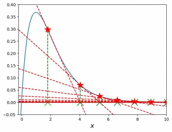
The red stars in this picture show where a tangent is attached to the blue curve of the function. The green Xs show where a tangent hits the x-axis, the tangents are the red dashed lines, and the green dashed lines connect each X to the next star.
For complex variables, we move along a two-dimensional surface instead of along a one-dimensional curve, but the principle is the same. The term in the denominator of the fraction of the iteration prescription, \(f'(x_i)\), is the reason for complex analysis being relevant for this problem.
By being able to define a derivative of a function also for complex arguments, we have the ability to choose not only real numbers for the initial guess, but also complex numbers. In this way, we work with a two-dimensional grid of numbers, the real and imaginary parts of those complex numbers. For each grid point we run Newton’s method and get information about which of the roots the method converges to from this particular starting point, and after how many steps. This outcome can be turned into a pretty picture.
You can imagine the steps from the initial guess on the grid, \(x_0\), going towards one of the positions of the roots in the complex plane, like following navigational instructions on a two-dimensional map. This map and path are different for each starting point on the grid, but what counts in the end is not the path, but only to which one of the roots the path leads from a particular \(x_0\).
One more thing: this path is the same for a particular \(x_0\) each time we start Newton’s method from there for a particular function \(f\). In this way, each function has its specific Newton fractal.
How to plot the graph of a Newton fractal
The graph of a Newton fractal is created by assigning different colors to the points on a grid of complex numbers, according to which one of the different roots of a function Newton’s method converges to from each grid point.
So the concrete steps are:
- Decide, which function \(f(x)\) to use; this determines the structure of the fractal. Whether it can look boring or super-exciting depends only on the choice for \(f\), see the examples below.
- Define the two-dimensional grid of points in the complex number plane. Each of those will serve as an initial guess to Newton’s method.
- Get a list of the roots of \(f(x)\), more precisely, their positions in the complex number plane with sufficient precision and accuracy.
- Actually, the list of roots need not necessarily be complete, but the more roots you have, the more colorful your picture will be.
- Run Newton’s method, starting from each grid point, and determine, to which one of the roots it is converging for this grid point. Also note after how many iteration steps a certain target precision is reached for each grid point.
- In the end, you’ll have a list of the following numbers for each grid point:
- An x-coordinate
- a y-coordinate
- the root to which Newton’s method converged (let’s ignore singular points in the procedure for this)
- how many iteration steps it took to reach the root with a given preset precision
Then all that is left to do is the following:
- Assigning a different numerical value to each of the roots, e.g., an integer index (you just number the roots)
- Turning this numerical value into a color
- Plotting the resulting colors for all the grid points
- If you like, you can use the number of necessary iteration steps to shade the color.
That’s it. When you do this, you should make sure of the following:
- The positions of the roots should be covered by your initial grid, at least partially. This isn’t necessary, but it is a good first version of your grid so that you can see, where interesting things happen. Then you can reset the grid to zoom or out or set positions as you like.
- You know how many steps on average it takes Newton’s method to converge on your grid. In this way, you can pick a suitable maximum number of iterations (setting such a maximum avoids infinite loops in your code).
- The precision you require of Newton’s method for each starting point should be higher than the precision, with which you decide that a result lies close enough to one of the roots. This identification of the finishing point with one of the roots is also done numerically.
- Start with a small enough number of grid points. Such computations can get lengthy very rapidly and you can always use more grid points, once you are certain that everything is working as expected.
Now I’ll stop with all the describing and get to the showing you stuff more concretely. Here come some examples:
Newton fractal example 1:
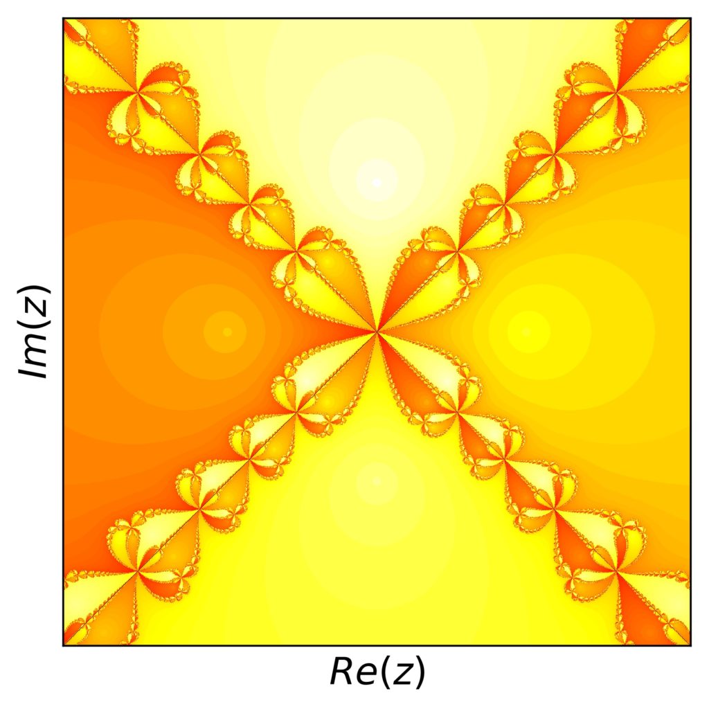
The first example I show you is a prominent one. The function is not the one above (that would be rather boring), but just a little bit more complex. We use, and now I write \(z\) instead of \(x\) to reflect that we are dealing with complex numbers:
\[f(z)=(z^2-1)(z^2+1)\]
Its derivative is
\[f'(z)=2 z \left((z^2-1)+ (z^2+1)\right)\]
and so the iteration becomes
\[z_{i+1}=z_i -\frac{ (z^2-1)(z^2+1)}{2 z \left((z^2-1)+ (z^2+1)\right)}\].
This function has four complex zeros:
\[-1,\;+1,\;-i,\;+i\;\]
which means that our fractal should have four different colors based on the convergence towards these four roots. We use a complex grid of \(z\) with 1000 values for real and imaginary parts each \(\in [-2,2]\). The result is:
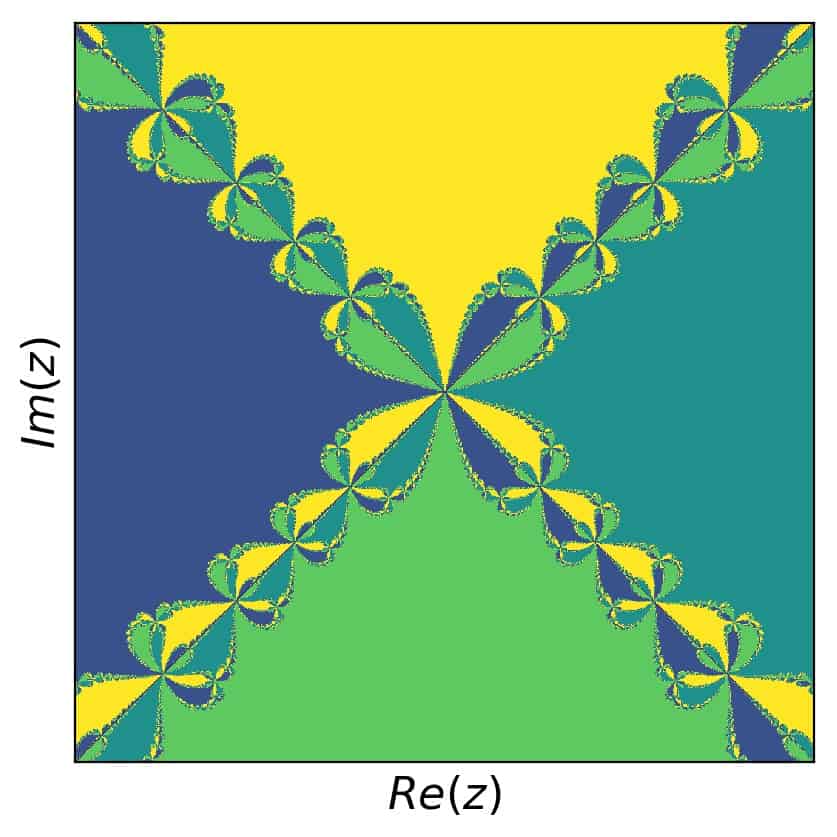
Now, in order to find self similar regions, we need to zoom in somewhere. Let’s focus on the the following range in real an imaginary parts first: \([0,0.7]\). This brings us to:
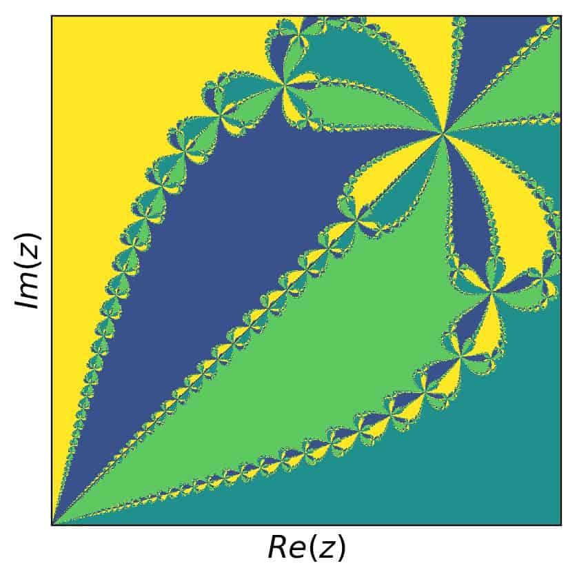
And now, zooming in to the real and imaginary parts with \([0.415,0.445]\), we get this picture:
Looks pretty similar, doesn’t it? In this concrete example, the same structure can be found in numerous places, as the images suggest. But you can also find different structure within themselves by selecting a portion of the picture and zooming in accordingly.
For your convenience, I have included the piece of python code that I used to create these pictures below at the bottom of this article. Feel free to use that to explore Newton fractals further.
And now on to another example.
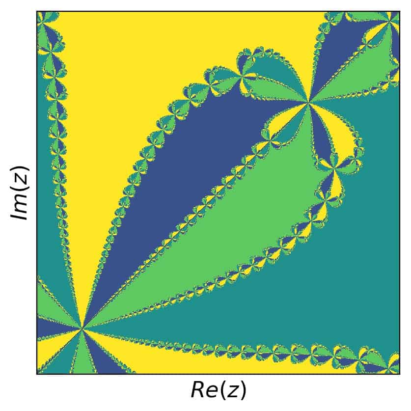
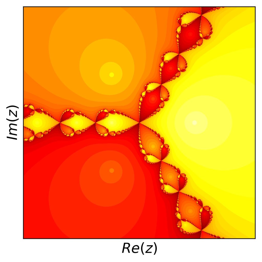
Newton fractal example 2:
For this second example, I’d like to use a polynomial as well. This time, the four roots are all real and the following:
\[-2, -1.5, 0.5, 2\]
As you can construct simply by multiplying the corresponding factors together, the polynomial with these roots is:
\[f(z)=(z-2)(z-0.5)(z+1.5)(z+2)\]
Taking the first derivative of this polynomial is simple. Just use the product rule and you’ll get the four terms (you can check in the python code example below). For a start, we set our initial grid to real and imaginary parts of \(z\) from the interval \([-2.1,2.1]\) in order to keep all roots inside the grid. Running the Newton-Raphson method and identifying each solution of the algorithm with the corresponding root, we get this picture:
In this case, we can also try to find self similar pieces, but it isn’t as obvious as in the previous example. Let’s zoom in on the region \([-0.8,-0.4]\) in the real and \([-0.2,0.2]\) in the imaginary part. Here is the result:
Then, we look at the region \([1.33,1.418]\) in the real and \([-0.04,0.04]\) in the imaginary part. Here is that result:
Not exactly the same, but you get the idea. What’s also interesting is to go and hunt for interesting and colorful detail. So here we go, for example with \([1.23,1.43]\) in the real and \([-0.1,0.1]\) in the imaginary part:
In general, polynomials can have a rich structure, depending on the number on positions of the roots. Just play with this yourself and you’ll sure enough discover a number of beautiful structures.
Newton fractal example 3:
Before we move beyond polynomials, I’d like to show you what happens, when one of the zeros is a multiple zero. In my article Highly Instructive Examples for the Newton Raphson Method I investigated this change, because multiple roots actually lead to slower speeds in convergence of the algorithm.
The function to investigate here is very similar to that in example 2 above. The only difference is a square on the third factor:
\[f(z)=(z-2)(z-0.5)(z+1.5)^2(z+2)\]
The roots remain the same, \(-2, -1.5, 0.5, 2\). The root at \(-1.5\) is a double root. Running the Newton-Raphson method and creating the fractal, we find the following picture:
What we can qualitatively say for the overview is that the region around the double root is larger than for the simple root. Looking for differences in the details, I recreated the last detail plot from the previous example with the changed function and found this, similar, but subtly different:
The structure has also been shifted a bit in the positive real direction. Once you experiment with various polynomials of different order, with different real and complex roots, and with multiple roots included, you will likely get a good feeling for what to use in order to get certain shapes, objects, and general structures.
Newton fractal example 4:
In the next example, we’ll move beyond polynomials. In principle this difference doesn’t change our approach to creating a Newton fractal. An interesting difference to note, though, is that, e.g., periodic functions like a sine function have infinitely many roots. Actually, let’s investigate the concrete example of
\[f(z)=\sin(z)\]
and
\[z_{i+1}=z_i – \tan(z_i)\].
The sine function has zeros at \(z=n \pi\), where \(n\) is an integer.
For our algorithm, this has the following consequence: In order to figure out, which root the Newton-Raphson method converges to when started at a particular \(z_0\) in the complex plane, we need to compare the converged result with an infinite set of roots – in principle.
At the same time, the further away from our starting point the finishing root is, the more steps it will take to get there. So, again in principle, we’d have to allow for a large (infinite) maximum number of iteration steps and compare to a really large set of roots.
In practice, this isn’t actually feasible. So what can we do? One possibility is to allow for a reasonably large but finite maximum numbers of iterations in the first place. In any numerical computation, it is not advisable to allow for loops without a hard cut-off number of maximum steps. So that is not only practical, but also a good idea from a computational standpoint.
Next, we can limit the number of roots that a converged result is compared to. This opens up the possibility that one of the converged results cannot be matched with a root in our predefined list of roots. In other words, it doesn’t correspond to one of the colors assigned to the different roots in the fractal picture. However, it is a good idea to have a backup color (like black) for those points that do not finish close enough to any of the given roots in any case.
It is always possible in numerics that something goes weirdly wrong in a way that requires a failsafe mechanism. So, we define that any \(z_0\) that cannot be identified with one of the roots that we list or allow should be colored black (or white or whatever special color you see fit). The rest, those \(z_0\) that are correctly matched with one of the roots that we have listed, get colored according to that root’s assigned color.
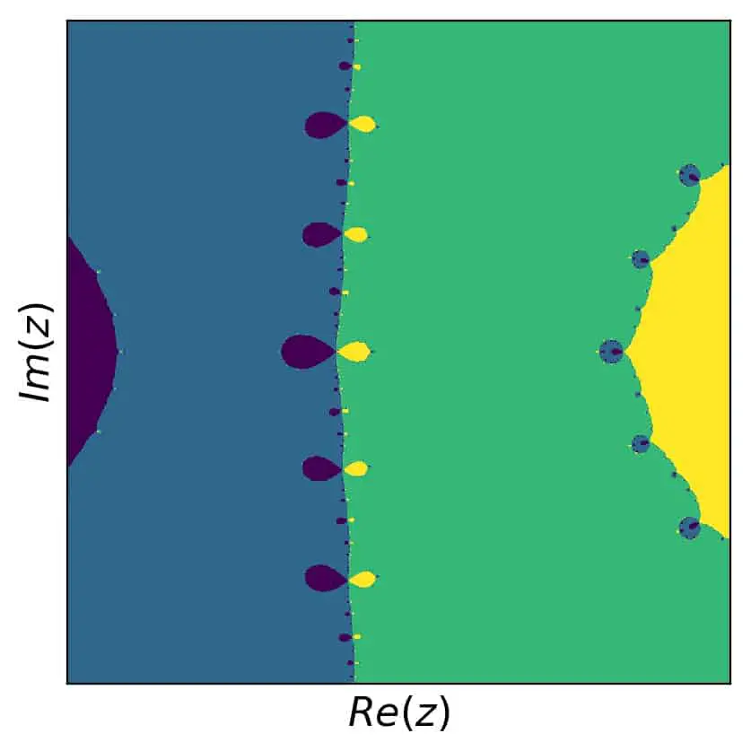
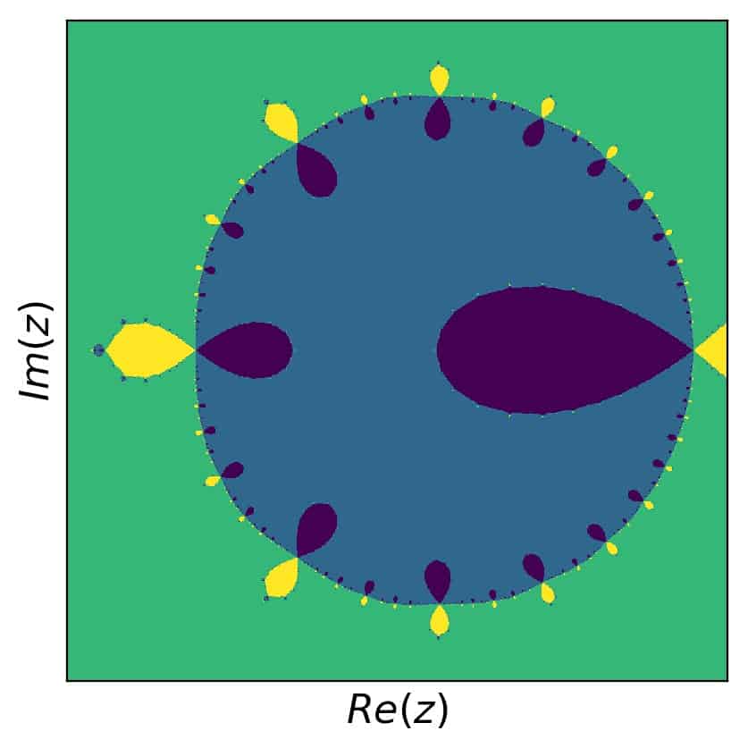
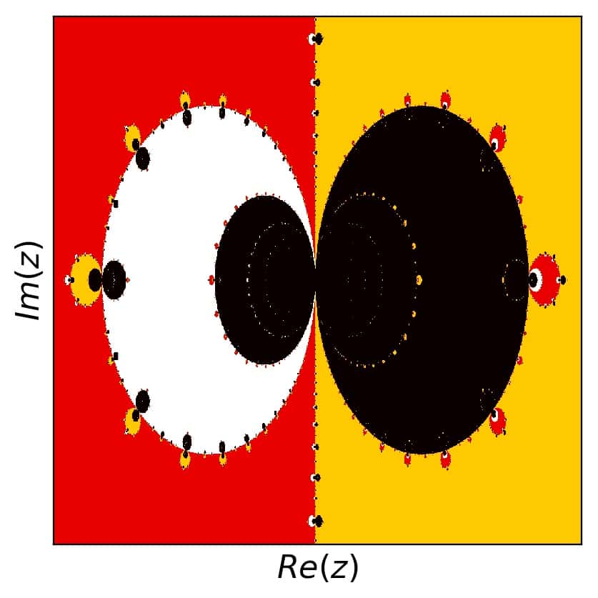
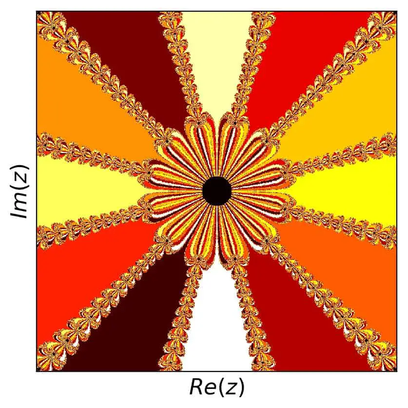
So what happens to the Newton fractal corresponding to the sine function, when we investigate this artificial dependence on the number of predefined roots? Let’s draw some pictures and find out. Here is the first try, with a maximum number of iterations set to 200 and only three roots:
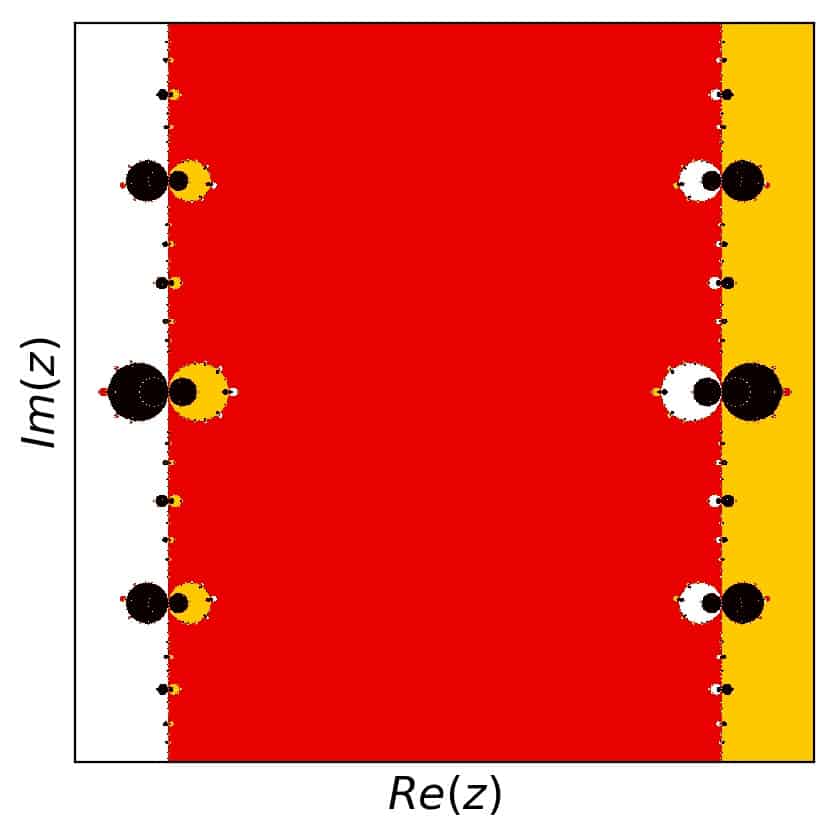
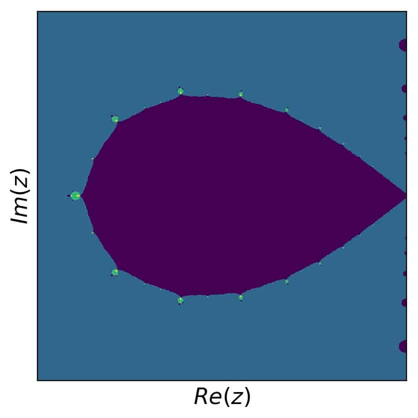
So there are four colors here: white for the root at \(z=-\pi\), red for the root at the origin, and yellow for the root at \(z=\pi\). The black color gets all the rest: the unmatched or unconverged points. Let’s plot the detail with \([1.15,2]\) in the real and \([-0.25,0.25]\) in the imaginary part as well, for some more insight:
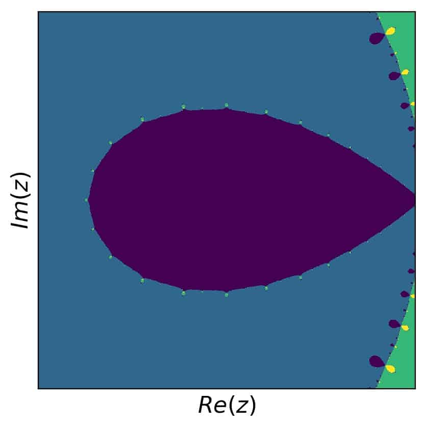
In these two pictures, there are hints toward a richer structure, if more roots are included. Not surprising, but worth exploring. So here we go. The same two pictures with 5 roots included are:
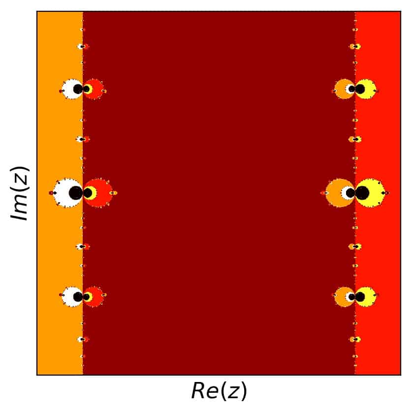
for the overview and
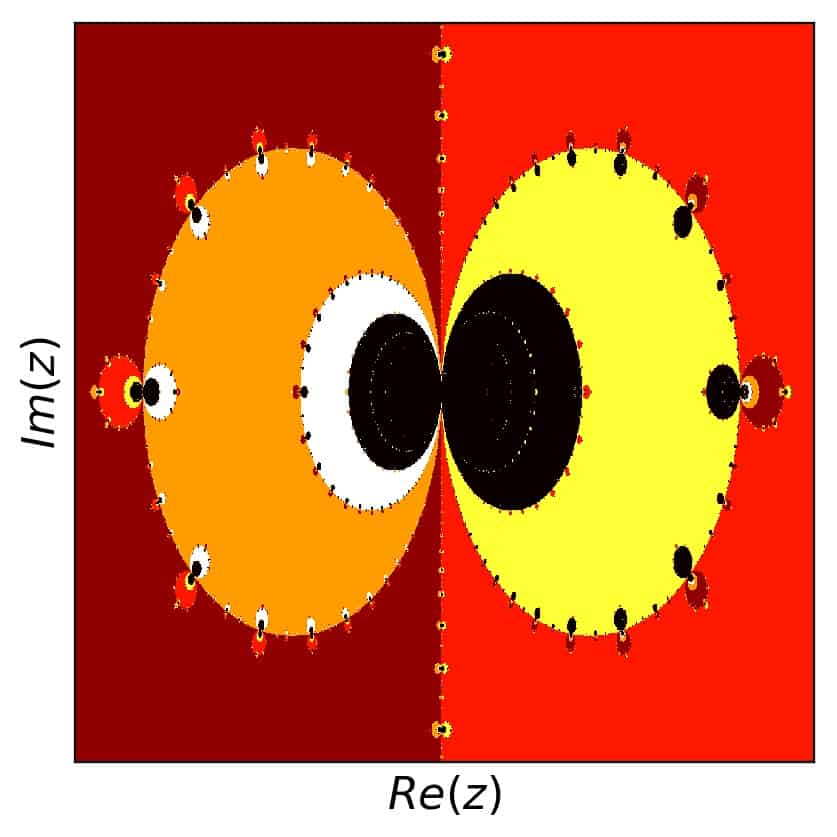
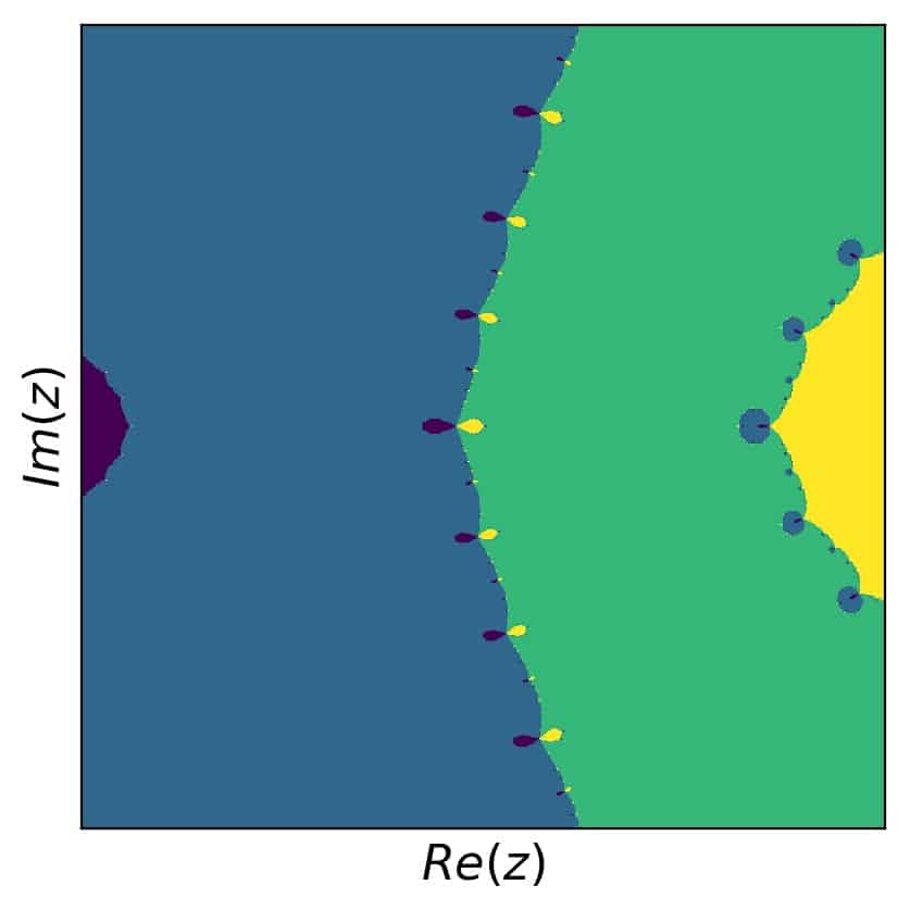
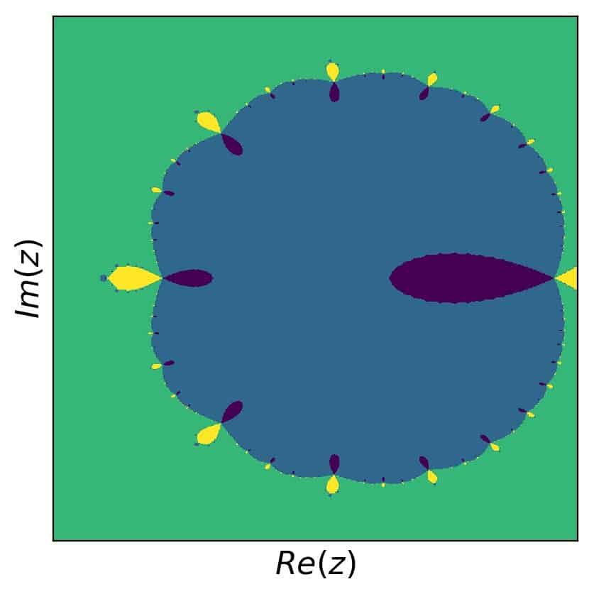
for our zoomed-in detail section. Now the plot includes two more colors, and we see that the boundaries that are somewhat visible within the black area in the middle actually separate areas that correspond to roots lying further out. Naturally, we’ll go to even more roots. However, let’s skip ahead to 11 roots, and let’s also skip the overview plot and focus on the detail, which shows the differences better. Here we are at 11 roots:
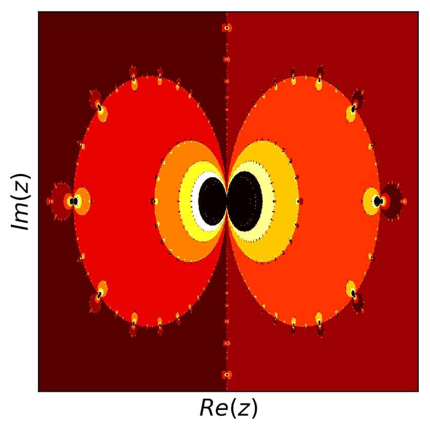
We can clearly see the inner black areas getting filled up with different colors everywhere in the picture. Let’s use even more roots. The detailed plot for 31 roots is up next.
And the pattern continues: the black area in the center, as well as all the other black parts, is filled up with even more colors. As a result, the color palette gets a bit stretched and the outer part of the picture turns darker, but I think it still looks good. Ok, one more with 51 roots:
More detail, more colors. By the way, if you’d like to create your own pictures like this and explore this effect and others even further, just use the python example code at the bottom of this article.
I think this rather nicely wraps our discussion of the Newton fractal corresponding to the sine function.
Newton fractal example 5:
As another example, I wanted to use something more complex. The interesting thing is that the sine example already showed quite a bit of complexity. While that was connected to the infinite number of roots of the sine, these roots were all aligned along the real axis.
In order to explore a bit more of the complex plane, let’s look at the following example function:
\[f(z)=z^{12}-1\]
Its derivative of this function is
\[f'(z)=12 z^{11}\]
and so we get for the iteration step
\[z_{i+1}=z_i -\frac{ z^{12}-1}{12 z^{11}}\].
This function has 12 real and complex zeros:
\[\pm 1,\;\pm i,\;\frac{\pm1\pm i\sqrt{3}}{2},\;\frac{\pm \sqrt{3}\pm i}{2}\]
which results in twelve different colors based on the convergence towards these roots. Since the complexity is a bit higher in this case, I used a complex grid of \(z\) with 2000 values for real and imaginary parts each \(\in [-2,2]\). The result is:
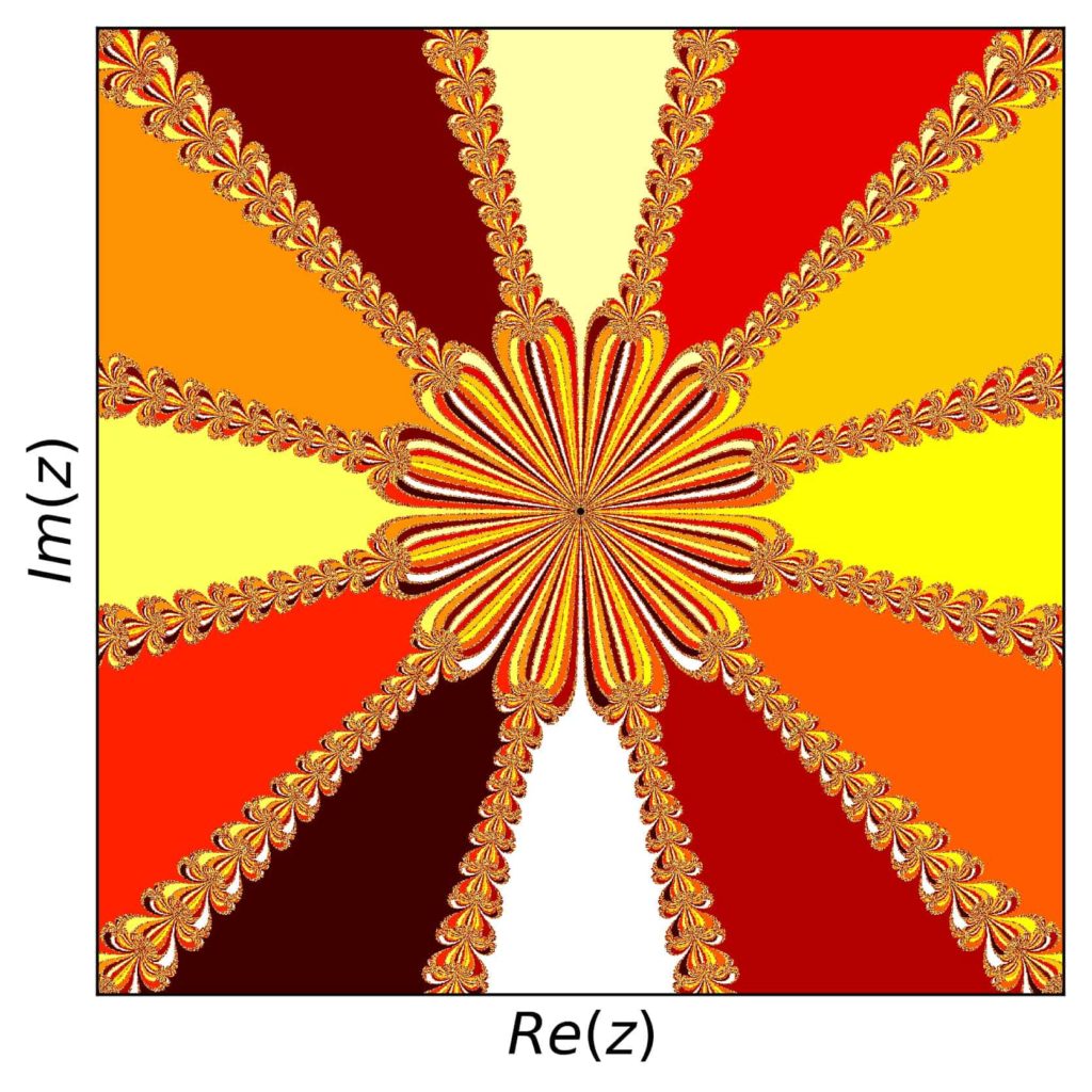
As for some nice detail, we can look at many places. Here is the view for \([0.48,0.8]\) both in the real and imaginary parts:
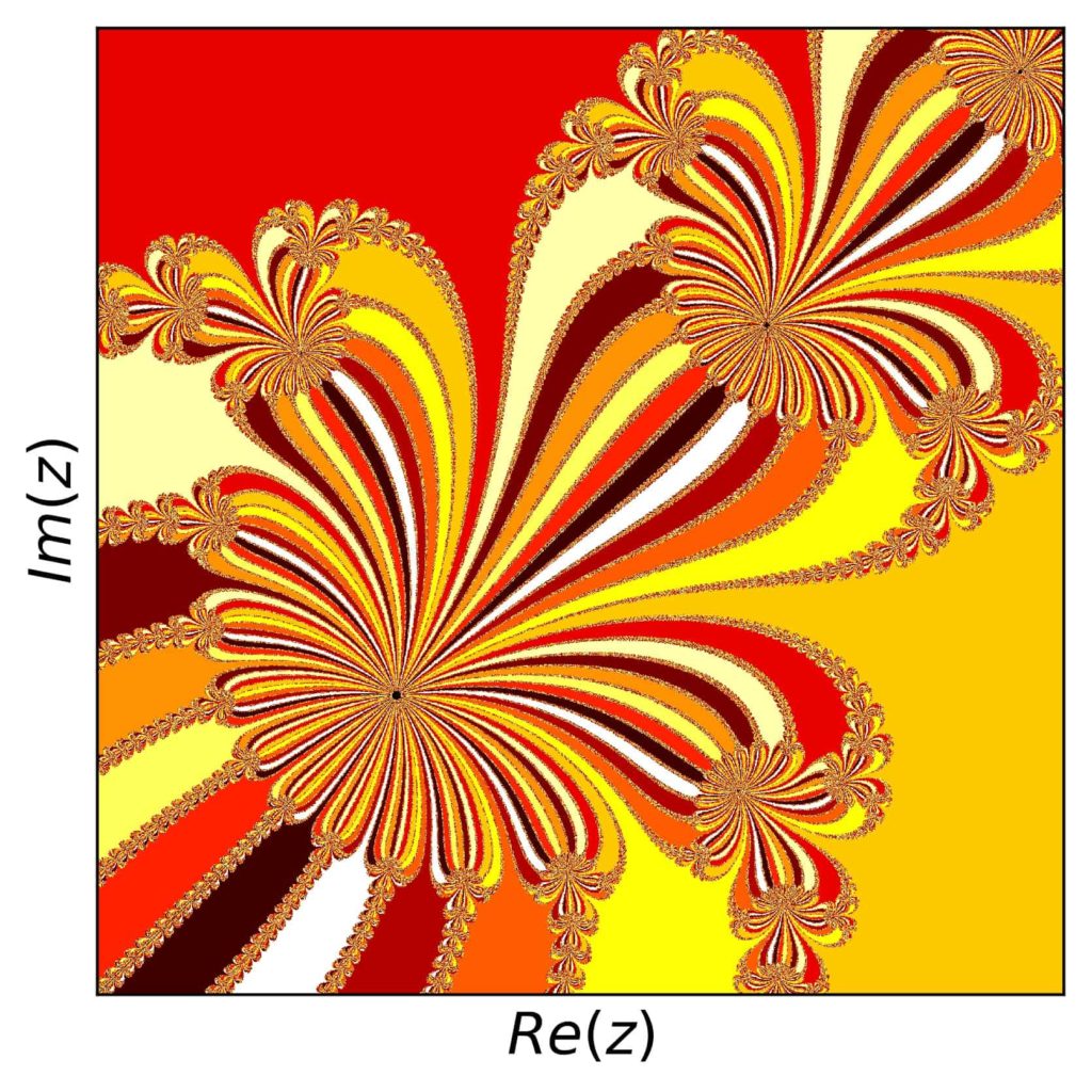
This is another example for the beauty and complexity of fractals, as it can be introduced by very simple functions or prescriptions.
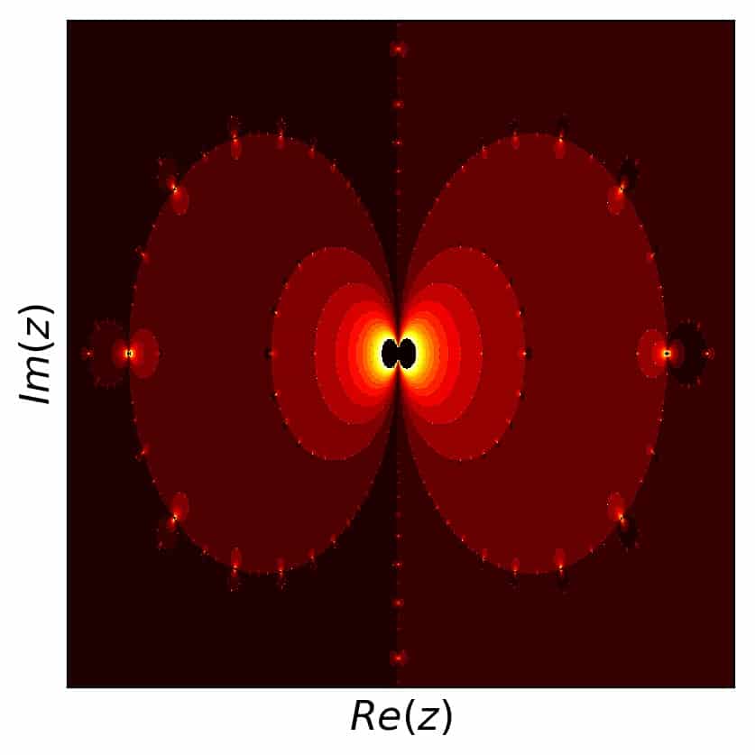
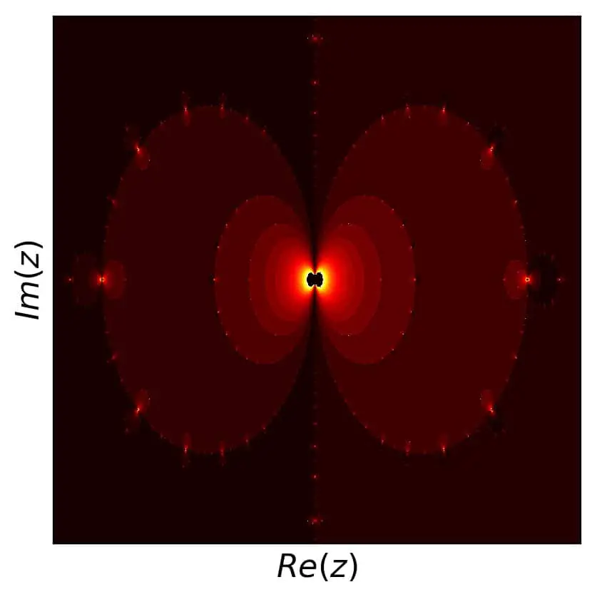
Including the number of necessary iterations in the plot
So far, we have only used colors in our fractal plots to indicate, which of the roots Newton’s method converges to for each grid point in the complex plane. But we still have some more information, namely the number of iteration steps it took for each case in order to reach a certain precision of the result.
This additional number can be used to give a Newton fractal a bit more detail in addition to the boundaries between regions corresponding to the different roots. If we shift the color for each point by an amount related to the number of necessary iterations starting at that point, we get a picture like this (for example number 1 above):
Note that I produced these pictures using a colormap in python’s matplotlib (see the code below). I shifted the color values such that the colors might actually mix across the different regions. Still, the result looks good, because the structure of a region with respect to the required number of iteration steps is well-behaved.
A similar change happens for our example number 5:
and for our example number two:
While I’d like to skip the sine function here, there is one more interesting case regarding the number of iterations required: our example with a multiple root, number 3. This comes from the fact that convergence is generally slower towards multiple roots than for simple ones. So let’s take a look:
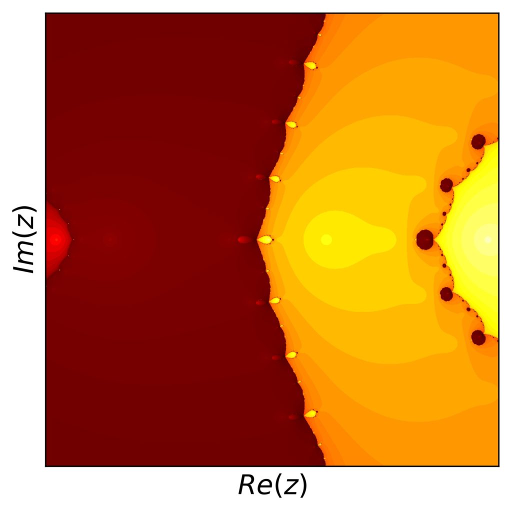
What we notice here is that the region around the double root (in the left middle of the picture) is substantially darker than the rest of the picture and so are the smaller regions throughout the complex plane that correspond to this root elsewhere.
As you’ll find in the code below and by thinking about it, there are many ways to take the number of necessary iterations into account in terms of producing a color shift. Playing with this can yield very interesting results.
List of Newton fractals
A list of Newton fractals would in practice correspond to a list of functions in one complex variable which have different roots such that the Newton method shows a fractal behavior depending on the starting point in the complex plane.
For obvious reasons, it isn’t feasible to go for a complete list of functions, but we have seen a couple of interesting examples here. What is a bit more straightforward, though, is to go for a list of different kinds of functions to use:
- a polynomial with all real roots
- a polynomial with complex roots
- a polynomial with roots on the unit circle
- a polynomial with a mix of simple and multiple roots
- trigonometric and other transcendental functions
- mixed functions of polynomials and trigonometric functions
In order to see some of these types and concrete picture examples for each , check the examples in this article. For some more examples (including some extensions of the method), I refer you to a little gallery on Wikipedia.
Python code example for the generation of Newton fractals
Finally, here is the python 3 code I used to create the pictures in this article. Feel free to use it for learning more about Newton fractals! If you are worried about a particular use that you have in mind, just read my short notes about my code examples here on ComputingSkillSet.com.
#!/usr/bin/env python3
# -*- coding: utf-8 -*-
"""
Created on Sat Sep 28 05:53:07 2019

Newton-Fractal example code.
Solves the Newton-method for a given function
on a grid of complex initial guesses.
Produces a color-coded graph of the fractal.
Includes several presets for function, but is easily extendable.

@author: Andreas Krassnigg, ComputingSkillSet.com/about/

This work is licensed under a
Creative Commons Attribution-ShareAlike 4.0 International License.
More information: https://creativecommons.org/licenses/by-sa/4.0/

"""

import matplotlib.pyplot as plt
import numpy as np
import datetime


# initialize a dictionary of list of the roots
rootlist = {}

# function definitions to evaluate f/f' at x. Add your own as needed.
# each function definition must include a list of the roots of this function
# root list can be in any order and restricted to finite number

# example 1: polynomial function with four roots
def npe1(x):
    return (x**2-1)*(x**2+1)/(2*x*(x**2-1)+2*x*(x**2+1))
rootlist['npe1'] = [-1, 1, -1j, 1j]


# example 2: function with three roots on the unit circle
def npe2(x):
    return (x**3-1)/(3*x**2)
rootlist['npe2'] = [-.5-0.8660254037844386j,-.5+0.8660254037844386j, 1]


# example 2: function with twelve roots on the unit circle
def npe3(x):
    return (x**12-1)/(12*x**11)
rootlist['npe3'] = [-.5-0.8660254037844386j,-.5+0.8660254037844386j,.5-0.8660254037844386j,.5+0.8660254037844386j,-.5j-0.8660254037844386,-.5j+0.8660254037844386,.5j-0.8660254037844386,.5j+0.8660254037844386, 1,-1,1.j,-1.j]


# example 7: function with four roots, all real
def npe7(x):
    return (x+2.)*(x+1.5)*(x-0.5)*(x-2.)/((x+1.5)*(x-0.5)*(x-2.) + (x+2.)*(x-0.5)*(x-2.) +(x+2.)*(x+1.5)*(x-2.) + (x+2.)*(x+1.5)*(x-0.5))
rootlist['npe7'] = [-2, -1.5, 0.5, 2]


# example 9: function with four roots, one multiple
def npe9(x):
    return (x+2)*(x+1.5)**2*(x-0.5)*(x-2)/((x+1.5)**2*(x-0.5)*(x-2) + 2*(x+2)*(x+1.5)*(x-0.5)*(x-2) +(x+2)*(x+1.5)**2*(x-2) + (x+2)*(x+1.5)**2*(x-0.5) )
rootlist['npe9'] = [-2, -1.5, 0.5, 2]


# example 10: sine function
def npe10(x):
    return np.tan(x)
rootlist['npe10'] = [0]
for i in range(1,10):
    rootlist['npe10'].extend([i*np.pi,-i*np.pi])


# define a function that can id a root from the rootlist
def id_root(zl,rlist):
    findgoal = 1.e-10 * np.ones(len(zl))
    rootid = -1 * np.ones(len(zl))
    for r in rlist:
        # check for closeness to each root in the list
        rootid = np.where(np.abs(zl-r* np.ones(len(zl))) < findgoal, np.ones(len(zl)) * rlist.index(r), rootid)

    return rootid


# define parameters for plotting - adjust these as needed for your function

# define left and right boundaries for plotting
# for overview plots:
interval_left = -2.1
interval_right = 2.1
interval_down = -2.1
interval_up = 2.1

# for detailed plots (adjust as needed):
#interval_left = 1.15
#interval_right = 2.
#interval_down = -0.25
#interval_up = 0.25

# set number of grid points on x and y axes for plotting
# use 100 for testing plotting ranges, 1000 for nice plots and 2000 for nicer plots
num_x = 1000
num_y = 1000

# set desired precision and max number of iterations
# keep precision goal smaller than findgoal (root matching) above
prec_goal = 1.e-11
# max number of iterations. Is being used in a vectorized way.
# 50 is a good minimal value, sometimes you need 500 or more
nmax = 200

# timing
print('Started computation at '+str(datetime.datetime.now()))


# define x and y grids of points for computation and plotting the fractal
xvals = np.linspace(interval_left, interval_right, num=num_x)
yvals = np.linspace(interval_down, interval_up, num=num_y)


# the following defines function to solve and plot. Jump to end of code to choose function
def plot_newton_fractal(func_string, perfom_shading=False):

    # create complex list of points from x and y values
    zlist = []
    for x in xvals:
        for y in yvals:
            zlist.append(x + 1j*y)

    # initialize the arrays for results, differences, loop counters
    reslist = np.array(zlist)
    reldiff = np.ones(len(reslist))
    counter = np.zeros(len(reslist)).astype(int)
    # initialize overall counter for controlling the while loop
    overallcounter = 0
    # vectorize the precision goal
    prec_goal_list = np.ones(len(reslist)) * prec_goal
    # iterate while precision goal is not met - vectorized
    while np.any(reldiff) > prec_goal and overallcounter < nmax:

        # call function as defined above and
        # compute iteration step, new x_i, and relative difference
        diff = eval(func_string+'(reslist)')
        z1list = reslist - diff
        reldiff = np.abs(diff/reslist)

        # reset the iteration
        reslist = z1list

        # increase the vectorized counter at each point, or not (if converged)
        counter = counter + np.greater(reldiff, prec_goal_list )
        # increase the control counter
        overallcounter += 1

    # get the converged roots matched up with those predefined in the root list
    nroot = id_root(z1list,rootlist[func_string]).astype(int)

    # add information about number of iterations to the rood id for shaded plotting
    if perfom_shading == True:
        nroot = nroot - 0.99*np.log(counter/np.max(counter))

    # uncomment those in case of doubt
#    print(reslist)
#    print(counter)
#    print(nroot)

    # get the data into the proper shape for plotting with matplotlib.pyplot.matshow
    nroot_contour = np.transpose(np.reshape(nroot,(num_x,num_y)))

    # timing to see difference in time used between calculation and plotting
    print('Finished computation at '+str(datetime.datetime.now()))

    # create an imshow plot
    plt.figure()

    #label the axes
    plt.xlabel("$Re(z)$", fontsize=16)
    plt.ylabel("$Im(z)$", fontsize=16)

    # plots the matrix of data in the current figure. Interpolation isn't wanted here.
    # Change color map (cmap) for various nice looks of your fractal
    plt.matshow(nroot_contour, fignum=0, interpolation='none', origin='lower', cmap='hot')

    # remove ticks and tick labels from the figure
    plt.xticks([])
    plt.yticks([])

    # save a file of you plot. 200 dpi is good to match 1000 plot points.
    # Increasing dpi produces more pixels, but not more plotting points.
    # Number of plotting points and pixels are best matched by inspection.
    plt.savefig('newton-fractal-example-plot-'+func_string+'.jpg', bbox_inches='tight', dpi=200)

    plt.close()
    # timing step
    print('Finished creating matshow plot at '+str(datetime.datetime.now()))


# call the solution function for func of your choice
# also, switch shading via number of iterations on or off
plot_newton_fractal('npe1', perfom_shading=True)

# final timing check
print('Finished computation and plotting at '+str(datetime.datetime.now()))
More information about Newton’s method
If you like this pictures and would like to understand better, what the algorithm behind it does, just click over to my articles Newton’s Method Explained: Details, Pictures, Python Code and Highly Instructive Examples for the Newton Raphson Method!