Newton’s method for numerically finding roots of an equation is most easily understood by example. At least, I learn more easily from examples. So, perhaps you do, too.
In this article I’ve collected a couple of highly instructive examples for the Newton-Raphson method and for what it does. You’ll see it work nicely and fail spectacularly. I show you the equations and pictures you need to understand what happens, and I give you a piece of python code so that you can try all that yourself.
Before we dive into the examples, let me mention that I have written a complete introduction to Newton’s method itself, here on ComputingSkillSet.com, in my article Newton’s Method Explained: Details, Pictures, Python Code. If at any step in one of the examples you feel like you could benefit from looking at an explanation of this particular step, just jump over there and come back afterwards.
And one more thing: Newton’s method for finding roots of a function is also called the Newton-Raphson method, so I’ll use these two names interchangeably.
Example 1: calculating square roots of positive numbers with Newton’s method
Newton’s method can be used to calculate the square root of a positive real number. Sounds interesting, doesn’t it? But how does this computational algorithm help to compute square roots? Here is how:
Let’s say that we are interested in the square root of 2. Then, we look at the function
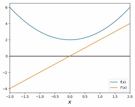
\[f(x)=x^2-2\]Why this function? Because the way Newton’s method works is that it can help us find zeros of functions, if we already have a faint idea as to where such a zero might be. In order to make use of this strategy, the function above is designed such that it has a zero at, yes indeed, the square root of two:
\[f(x)=0\quad\rightarrow\quad x^2-2=0\quad\rightarrow\quad x^2=2\]
This means that if we use Newton’s method to find the zero (root) of this function, it will give us a numerical value of the square root of two. At this point, it is already clear, by the way, what to do, if you’d want the square root of seven instead: You’d use \(f(x)=x^2-7\). But because we want to see a number come out that many people recognize, let’s stick to the square root of two.
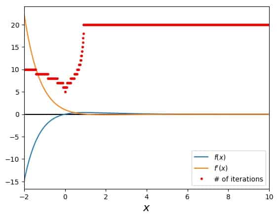
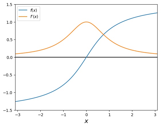
Here is an overview of what this function and its derivative look like:
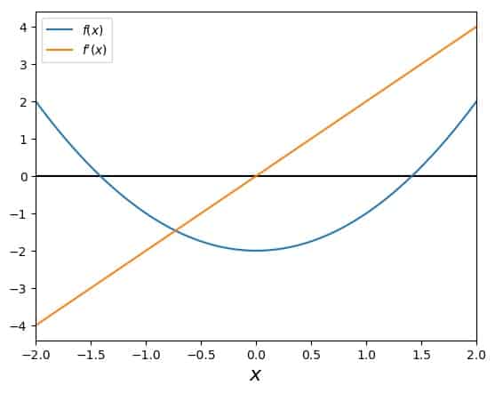
Newton’s method tells you to start with an initial guess, \(x_0\), and then iterate the following line until you are either satisfied with the result or the algorithm fails:
\[x_{i+1}= x_i – \frac{f(x_i)}{f'(x_i)} \]
For our concrete example function, this becomes
\[x_{i+1}= x_i – \frac{x_i^2-2}{2x_i} \]
and that is fairly easy to do, even by hand, if we’d like.
Ok, first we pick an initial guess. We know (playing naive on purpose here) that the square root of two lies somewhere between the numbers 1 and 2, so let’s pick \(x_0=1.5\), that’s right in the middle. Then we get
\[x_1= 1.5 – \frac{1.5^2-2}{3}= 1.5 – \frac{2.25-2}{3}= 1.5 – \frac{0.25}{3}=1.5 -0.0833333= 1.4166666 \]
So this is the first step. One thing that we need to keep an eye on is the relative difference in the \(x_i\) from one step to the next, namely:
\[\frac{|x_{i+1}- x_i|}{|x_i|}= \frac{|f(x_i)|}{|f'(x_i)x_i|} \]
For our particular example and step, we have
\[\frac{|f(x_0)|}{|f'(x_0)x_0|}=0.0555555 \]
Ok, next step. This time, doing the calculation without a calculator isn’t so much fun anymore, but I’ll still note the numbers as if we’d do it that way:
\[x_2= 1.4166666 – \frac{1.4166666^2-2}{2.8333333}= 1.416666666 – 0.00245098= 1.414215686 \]
To those of you who know the answer by heart, this should already look pretty good. To keep our score, let’s check the relative difference. It is
\[\frac{|f(x_1)|}{|f'(x_1)x_1|}=0.0017301 \]
On to the next step. We get
\[x_3= 1.414215686275 – \frac{1.414215686275^2-2}{2.828427137255}= 1.414215686275 – 0.000002123900= 1.414213562375 \]
You have certainly noticed that I keep adding more and more digits to those numbers, and that’s because it is necessary. The result is getting closer to the actual root of our equation really quickly now. Let’s note the relative difference for this step:
\[\frac{|f(x_2)|}{|f'(x_2)x_2|}=0.0000015 \]
So, because the next step should (and will) be smaller than this one, we can estimate that our result is already precise to 5 digits or more. One more step, ok? Here we go:
\[x_3= 1.414213562375 – \frac{1.414213562375^2-2}{2.82842712475}= 1.414213562375 – 0.000000000002= 1.414213562373 \]
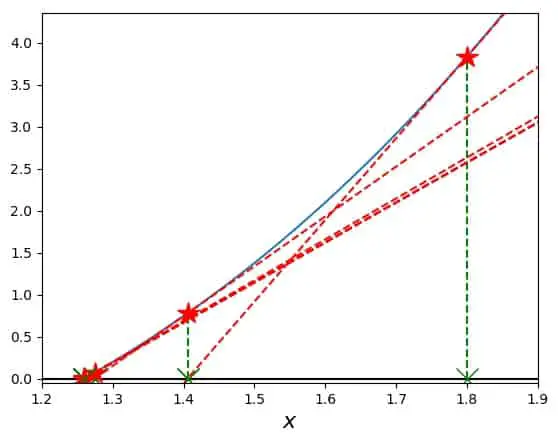
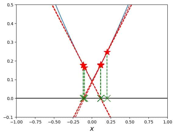
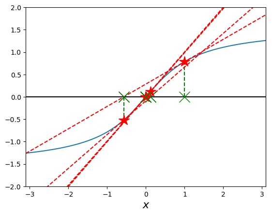
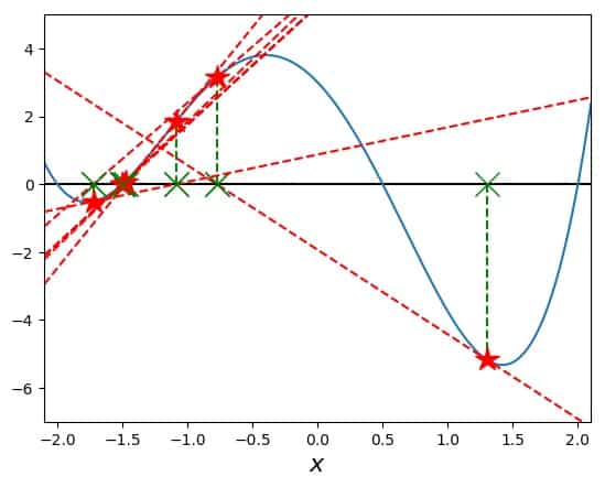
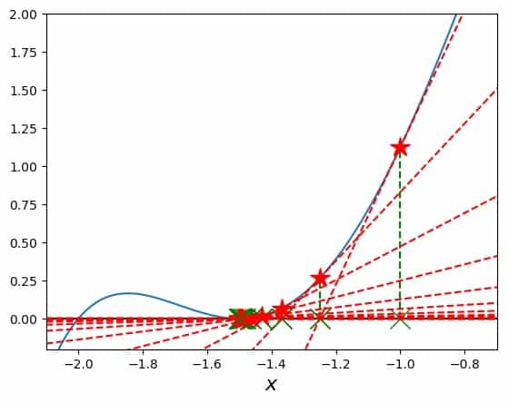
Just a tiny change. In fact, the relative difference is \(0.000000000001\) and we are done. This worked really well and fairly quickly, because we were close to the root and the function is well-behaved. To illustrate this, here is a plot of the tangents that were constructed to go these steps. All of them are very close and it is hard to see anything:
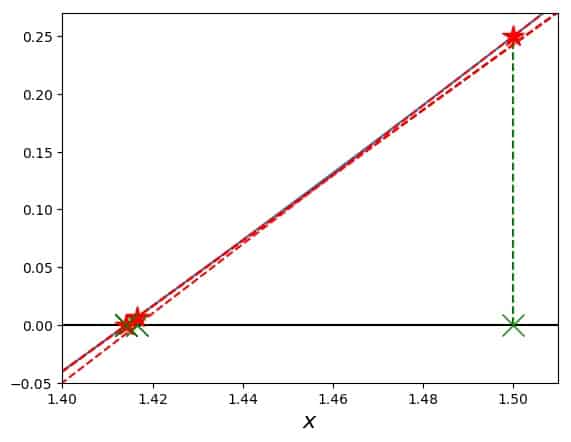
The function is plotted in blue and hard to see underneath the red-dashed tangents. The red stars mark those points on the curve, where the steps are. The green Xs mark the same points on the x-axis, and green dashed lines lead up to the respective stars.
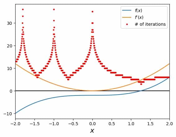
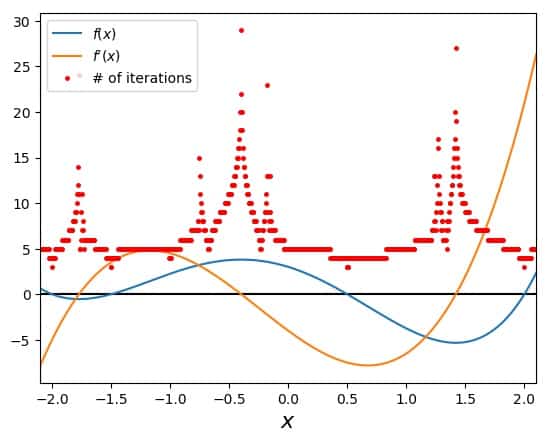
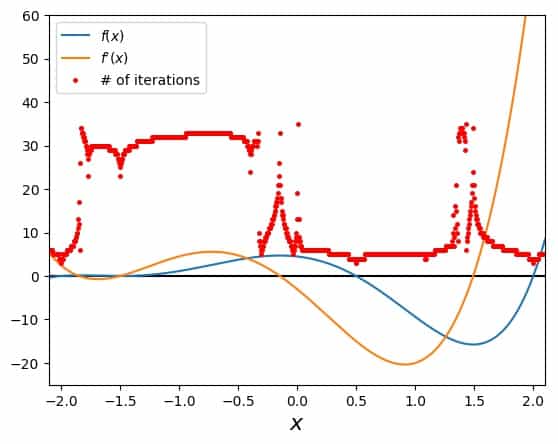
While for this particular choice of the initial guess, the convergence is fast, it is different for other initial guesses. To get an idea, how different it is, we can plot the number of iterations steps needed in order to reach a certain level of relative precision, in our case \(10^{-10}\). The result is the following figure:
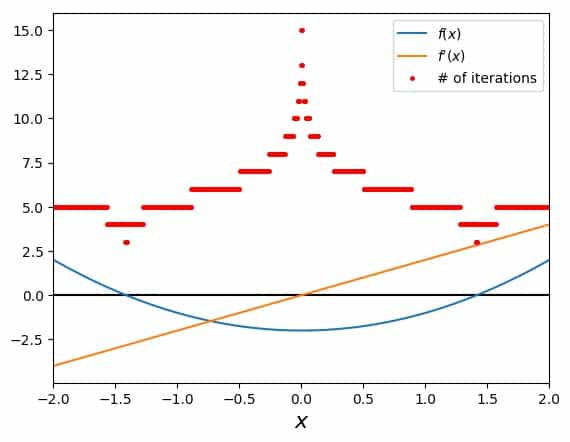
These red dots indicate areas of fast convergence, where they are low, and slow convergence, where they are high. In general, a small slope of the function in question at a certain initial guess leads to slower convergence. In our example, the origin is particularly unsuitable, because there the slope vanishes and so the Newton algorithm fails.
In summary, we have seen that Newton’s method can be used for getting numerical values for square roots of positive real numbers in a straightforward manner.
Example 2: calculating cubic roots of positive numbers with Newton’s method
This next example is similar to the first, but would be a little more annoying to do by hand. We’ll use the Newton-Raphson method to compute the cubic root of the number 2. This is a number that isn’t as familiar as the square root of two, but it is easy enough to check on a pocket calculator that can do cubic roots. So here we go.
The function we define for this purpose is (can you guess it after having read the first example?):
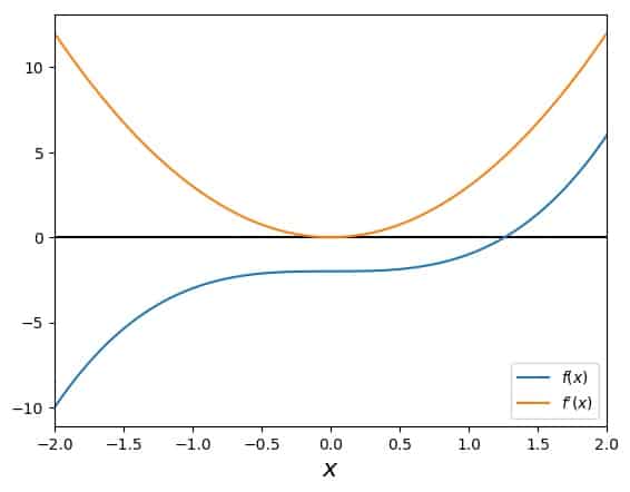
\[f(x)=x^3-2\]This function has the property of having a (single) root at \(x=\sqrt[3]{2}\), which is what we want to know and what Newton’s method will help us find. The function and its derivative look like this:
To start the search, let’s pick an initial guess, say \(x_0 = 1.8\). With the general formula
\[x_{i+1}= x_i – \frac{f(x_i)}{f'(x_i)} \]
we find for our cubic-root generating function
\[x_{i+1}= x_i – \frac{x_i^3-2}{3x_i^2} \]
Applying this to \(x_0 = 1.8\), we arrive at \(x_1 = 1.405761316872\) and a relative difference of \(0.219021490626\). Repeating the procedure (for more details, see example 1 above), we get \(x_2 = 1.274527978340\) with a relative difference of \(0.093353926415\), \(x_3 = 1.260087815373\) with a relative difference of \(0.011329812458\), \(x_4 = 1.259921071964\) with a relative difference of \(0.000132326816\), \(x_5 = 1.259921049895\) with a relative difference of \(0.000000017517\), and \(x_6 = 1.259921049895\) with a relative difference of \(0.000000000000\). Yes, that’s right – the last step didn’t change anything in the digits shown here. So that is our result:
\[\sqrt[3]{2}=1.259921049895\]
In a picture, these steps can again be visualized by the tangents that correspond to them:
In this case, at least the first tow steps and tangents are clearly distinguishable from the rest, before the plot becomes crowded near the actual value of the root. Again, we can ask about the dependence of the number of necessary steps on the initial guess. Testing this and plotting this number across the entire range plotted in the overview, we get:
The low regions in the red-dot-curve provide a good solution after a low number of iteration steps, while the high regions take longer. The point to avoid is once again the origin, where the slope of our function vanishes and the algorithm of the Newton-Raphson method stops.
Example 3: calculating any roots of positive numbers with Newton’s method
This example also deals with calculating roots, but I’d like to keep this brief. You already got the idea from the first two with the concrete numbers and the illustrations. In this example, I want to just write down the general formula for computing the \(n^{th}\) root of the number \(a\).
In order to find a number that is the \(n^{th}\) root (\(n>1\)) of the positive real number \(a\), which function do we need to use in Newton’s method? We use
\[f(x)=x^n-a\]because this is zero, where \(x=\sqrt[n]{a}\). Now, recall the Newton-Raphson iteration step, which is
\[x_{i+1}= x_i – \frac{f(x_i)}{f'(x_i)} \]
and substitute for \(f\) and \(f’\) accoringly. That brings us to
\[x_{i+1}= x_i – \frac{x_i^n-a}{n x_i^{n-1}} \]
In much the same way, we can construct the iteration step explicitly in terms of the function we want to investigate. This works, provided that we can write down a functional form for the function and its derivative.
In the next couple examples, we’ll see and experience the various ways, in which Newton’s method can and will fail.
Example 4: Newton’s method fails when there is no root
In my article Newton’s Method Explained: Details, Pictures, Python Code, I mention a number of cases where Newton’s method can or will fail. In the following, I present some examples for exactly those cases. The first of these is that the function, for which we try to find a root, doesn’t actually have any.
Now you might say that this is an artificial situation, because we usually know whether the functions we investigate have roots or not. While this is true for something like \(f(x)=x^2\), it can indeed be more complicated in general.
Think about the following situation: you tell me about some interesting phenomenon. We figure out an equation together that’s supposed to describe this phenomenon. But our equation isn’t algebraic to begin with, so we have no idea what the solution looks like, we just know that it should be a function of a single variable, whose most important part is its zero (root). So in the first step, we need to calculate the function for which we’d like to use Newton’s method. And then it could well happen that there is no root for this function. Ok, enough with the mind experiments, let’s look at an example.
Above, we have used the function
\[f(x)=x^2-2\]for computing the square root of two, because we know that its root is the number we want. If we “shift this function up” by adding the number four to it, we get
\[f(x)=x^2+2\]and there isn’t any (real) root any more. So, let’s try Newton’s method on this and see what happens. The function and its derivative look like this:
Here we can clearly see that the function (in blue) doesn’t even come near zero. Its derivative is problematic in the same fashion as above, i.e., there is a zero value for the slope at the origin.
I started Newton’s method at \(x_0=1.8\) and gave it 10 steps to try and find a solution (remember that this was enough in the square-root-finding example above), but (obviously), the algorithm just keeps wandering around:
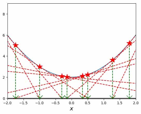
In order to see immediately that just using more steps doesn’t (because it cannot) help, here is the same plot again, but this time with ten times as many possible steps, i.e. 100 maximum iterations:
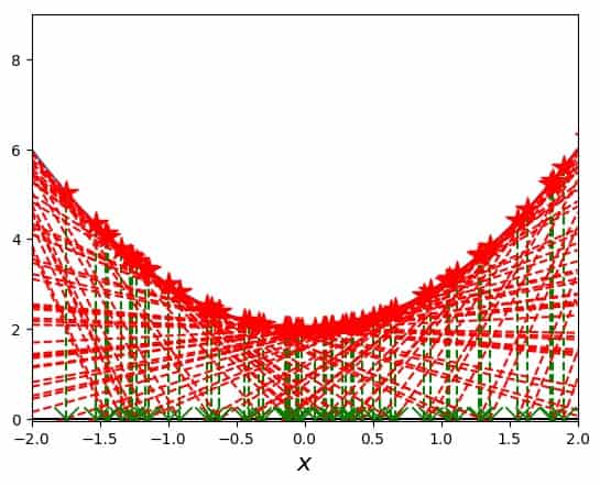
So, there are 100 tangents in this picture (or maybe not all of them actually show up between \(x=-2\) and \(x=2\). You can see a lot of them, that’s good enough. So, if your Newton-Raphson iteration does not converge and you don’t know why, this case is one possibility.
Example 5: Newton’s method running away into an asymptotic region of the function
Another possible failure of Newton’s method happens, when there is an asymptotic region in the function, e.g., the function falls off monotonously towards positive infinity, but doesn’t reach zero. What? Let’s look at a concrete example. We’ll use the function
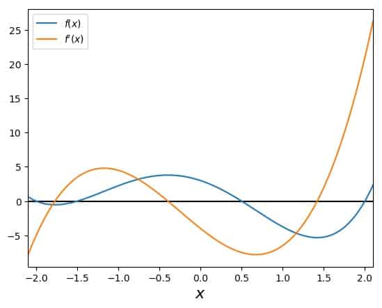
\[f(x)=x \exp(-x)\]which has such an asymptotic region towards positive infinity. Here it is plotted together with its derivative:
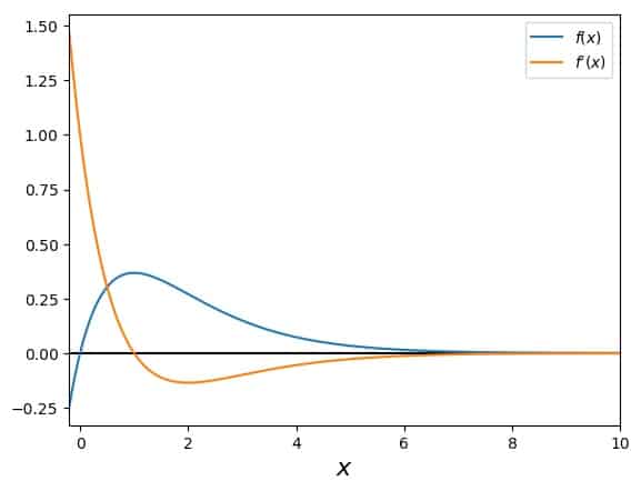
We can see clearly that the function actually does have a root, which the Newton-Raphson method can also find, but only if it starts at a suitable point. Our choice of \(x_0=1.8\), for example lies near the maximum of the function, more precisely, to the right of the maximum. If a search for a root with Newton’s method starts there, the following happens:
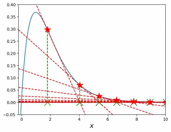
We observe that the slope to the right of the maximum is always negative. So, once the method starts there, the \(x_i\) can only move to larger and larger numbers and their sequence actually diverges spectacularly.
If, on the other hand, the search is started left of the maximum, say at \(x_0=0.5\), the method finds the root after 6 iteration steps. Here is the graph with the iteration path laid out by the red stars on the curves and the green Xs on the x-axis:
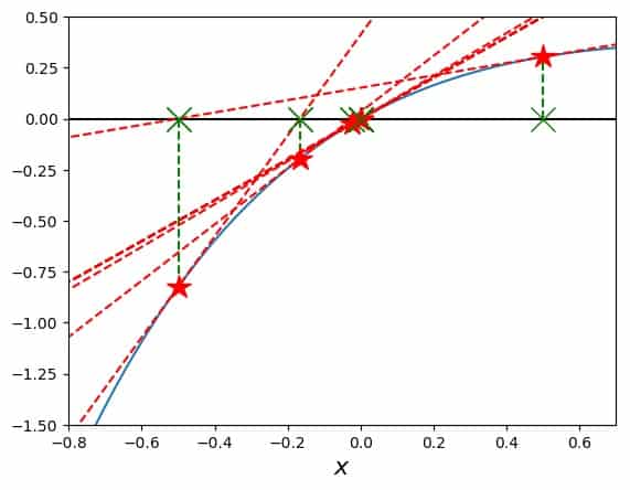
I should mention here that converging towards a solution of zero (as it happens here) is a little problematic when defined via a relative difference. Once the level of precision of the root is such that it appears as zero in the computer’s memory, a division by zero is encountered. However, meaningful values are produced on the way to this failure, so we can still feel content about having avoided the asymptotic trap of this function.
For this case, I show the third kind of plot again (like in the first example), where the number of iteration steps needed for a solution is added to the overview. Here it is:
The red dots show the (obviously discrete) values for the number of necessary iterations, if Newton’s method is started at this value for \(x_0\). Keep in mind that there is a maximum number of iterations in my code in order to avoid an infinite loop when the algorithm fails to converge and stop. In this plot I set that maximum number to 20.
We can clearly see that a plateau at 20 appears at the maximum value of our function and is there for the entire asymptotic region of the exponential tail. To the left of the maximum of \(f\), there is our usual stuff: fewer iterations closer to the root.
To summarize this example: if you see your values for the \(x_i\) run away in one direction, maybe that’s the fault of an asymptotic region that your function shows there.
Example 6: Newton’s method oscillating between two regions forever
Another possibility for Newton’s method to get stuck in an infinite search pattern is an oscillation. In particular, in such a case the iteration procedure with the tangents jumps between two regions, whose slopes “point at each other”. Now what is that supposed to mean? Let’s check out an example.
A possible function that will show us this behavior is
\[f(x)=-\cos\left(|x|+\frac{\pi}{4}\right) + 0.8\]whose first derivative is
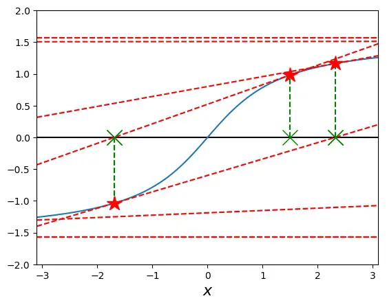
\[f'(x)=\sin\left(|x|+\frac{\pi}{4}\right)\; \text{sgn}(x)\]This is still hard to imagine just inside your head, so let me show you the graph of these two:
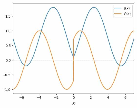
The interesting region for our purposes is in the middle, where the curvature is positive. Any Newton search in there will get trapped and cannot get out, for example:
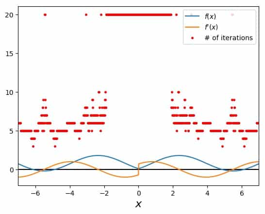
What does that mean for the convergence regions of Newton’s method for this function? There is a region in the middle, around the origin, where the method fails. Outside of that it works most of the time, but fails, where the one of the steps in the iteration leads into the “oscillation trap” in the center:
This may seem like an untypical case due to the function construction with the absolute value. However, the absolute value is not as uncommon as we would perhaps think or like.
So if you see your Newton method’s points oscillate (in sign or otherwise), then something like the case shown here might be happening.
Example 7: Newton’s method fails for roots rising slower than a square root
There are roots to which Newton’s method does not converge, but it diverges away from. Why? Because the function’s slope and curvature at the root produce iteration steps that go further and further away from the root, even if the initial guess is chosen very close to it.
The “border” behavior of the function in question for this to happen is that of a square root, i.e., if \(f(x)\) at the root rises more slowly than
\[f(x)=\sqrt{x}\]
then Newton’s method diverges away from the root. Let’s try this by investigating the cubic-root function:
\[f(x)=\sqrt[3]{x}\]
In this case, the derivative is
\[f'(x)=\frac{1}{3 x^{2/3}}\]
and the iteration step becomes
\[x_{i+1}=x_i – 3x_i=-2x_i\;.\]
Now, for this example we know that the root is located at \(x=0\). That means that, looking at the iteration step, we see how the \(x_i\) alternates in sign and grows in size at each step, i.e., it moves away from the root at zero.
Numerically, in this particular example, the initial guess gets multiplied by a factor of negative two at each iteration step, growing geometrically beyond all bounds. As a result, running this as a numerical exercise can only help to expose missing maximum numbers of iteration, or producing numerical overflows.
Example 8: Newton’s method for the arctangent function
A similar example, but with a region of convergence in the center, is the arctangent function:
\[f(x)=\arctan(x)\]
with the derivative
\[f'(x)=\frac{1}{x^2+1}\]
In this case the iteration step becomes
\[x_{i+1}=x_i – (x_i^2+1) \arctan(x_i)\;.\]
Now, for choices of \(x_0\) close enough to the origin, we get a converging pattern, e.g., for \(x_0=1\):
However, if we start a bit further away from the origin, say at 1.5, Newton’s method diverges spectacularly:
Here, the method oscillates and diverges away from the origin, producing a number larger than the computer can handle in less than 20 steps.
The boundary between these two regions (of convergence vs. divergence) can be found by solving the equation \(x_{i+1}=-x_i\), since the resulting sequence is alternating in sign. We find
\[x_i – (x_i^2+1) \arctan(x_i)=-x_i\]
and, simplifying the equation,
\[\arctan (x_i)=\frac{2x_i}{x_i^2+1}\]
whose solution is approximately \(1.39175\). If the absolute value of the initial guess is larger than this number, Newton’s method diverges, for smaller absolute values of the initial guess, it converges.
Example 9: A couple of roots to choose from for Newton’s method
Among all these examples for the use of Newton’s method to find roots of a function, we haven’t seen the most usual yet. So far, we’ve had cases with one root, no root, but not several roots. We’ve seen the method fail, but sometimes, the problem is not that it fails, but that it fails to find the solution that we want it to find. Sounds complicated? It can be. Here is an example.
For this purpose, a polynomial is kind of ideal: it is easily constructed, can have several roots at specific locations, and derivatives are simple to get, too. So let’s use
\[f(x)=(x+2)(x+1.5)(x-0.5)(x-2)\]with the first derivative
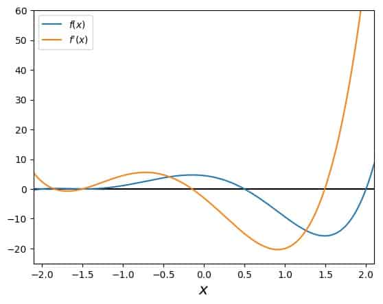
\[f'(x)=(x+1.5)(x-0.5)(x-2)+(x+2)(x-0.5)(x-2)+(x+2)(x+1.5)(x-2)+(x+2)(x+1.5)(x-0.5)\]These two look like this:
One can clearly see the four roots in the function, and that the derivative has three zeros, where Newton’s method will stop, if they are hit exactly. Other than that, there are no obvious problems. The convergence plot (which shows the number of iterations needed to arrive at a converged solution as red dots for each \(x_0\)) indicates exactly what I just stated: Nice convergence everywhere, except when hitting a zero in the first derivative.
Still, it is an interesting case for the following reason: Let’s try and compute the root at \(x=0.5\). And let’s pretend that this function is actually unknown to us in detail (playing stupid for demonstration purposes). We somehow figure that the value \(x_0=1\) would be a good idea, so we start a run of Newton’s method with this initial guess. Here is the resulting search with all the tangents:

Wow, this worked nicely! We found a root, and even better, we found our target! But what happens, if we don’t get so lucky, and someone had suggested \(x_0=1.3\)? Here is what happens:
Wow again, but in a different way! This search jumped to another root than the one closest to our starting point. And moving further to more positive starting values would bring it to the even further negative root at \(x=-2\). Then, just a little further, it would converge towards the most positive root at \(x=2\). So, you see that little differences in the initial guess can make quite a large difference in terms of where Newton’s method goes with its search pattern.
As a consequence, we should always try to get as close as possible to a root with our initial guess!
Example 10: Fractals generated with Newton’s method
Yes, indeed, there are fractals that can be generated by using Newton’s method. In short, the background is this: Although I kept stressing above at some places that we are looking for real roots, Newton’s method can be generalized to the complex plane (i.e., for complex numbers and functions).
If a function is well-behaved enough also for complex arguments, then we can also extend the validity of its derivative away from the real axis. If this is too much information for you, don’t worry. Just imagine that you are computing a derivative of a function with two real variables instead of one.
Now, how and why do fractals connect to Newton’s method and vice versa? The answer lies in the previous example. There, we have seen that Newton’s method can converge to different roots of a function from neighboring initial guesses \(x_0\). So far, we have only looked at the number of iterations it takes to arrive at a converged solution – any solution.
But now imagine that we are color-coding each \(x_0\), depending on which root of \(f\) the iteration converges to. So, if there are four roots, like in the previous example, there would be four colors. And then, we run Newton’s method, starting from each point on a two-dimensional grid of complex numbers.
We observe two things: to which root the method converges and how many iterations it takes to get there. The first (which root) is translated into the color of the starting point on the grid, and the second (how many iterations) can be used to additionally shade the color of that point.
I know this is a bit much all at once, which is why I have written an entire article in addition to this one, just about Newton fractals. You can find it here: Newton Fractals Explained: Examples and Python Code. Here is a sneak peek of such a fractal. The particular example is the one we used above as example number 7:
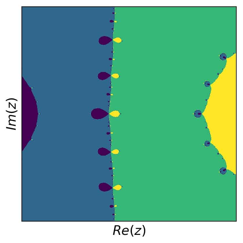
As you can see, this picture uses only color information and not shading – I leave the latter to the in-depth article linked above.
Example 11: Finding roots with higher multiplicity in polynomials with Newton’s method
Another typical example in connection with Newton’s method is the presence of multiple roots among the roots of a polynomial. So far, we have seen only simple roots in our examples. At this point, I’d like to show you one more with a double root. We’ll just reuse the function from example 7, but with a small difference:
\[f(x)=(x+2)(x+1.5)^2(x-0.5)(x-2)\]Note that the second factor is squared now, which means that the root of this polynomial at \(x=-1.5\) is now double. The first derivative reflects this as well and becomes
\[f'(x)=(x+1.5)^2(x-0.5)(x-2)+2(x+2)(x+1.5)(x-0.5)(x-2)+(x+2)(x+1.5)^2(x-2)+(x+2)(x+1.5)^2(x-0.5)\]The graphs of our function and its first derivative look similar to the one above in example 7, but a bit different:
Admittedly, it is hard to see the region around the double root, so we’ll go right into the search plot. Starting at \(x_0=-1\), we arrive at the desired solution:
Here one can see the graph of the function better around the double root. We also see how the tangents, stars and Xs are moving towards the solution. What isn’t evident from this figure, but is important and the reason for this example, is the speed of convergence towards the double root as compared to a single root.
For this, our usual plot with the number of necessary iterations as a function of the starting point comes in handy. Here it is:
Apart from the occasional jitter around the zeros of the first derivative, there are two clearly different regions with regard to the number of necessary iterations. The region around the double root at \(x=-1.5\) and everything else, which we can explicitly call “regions around simple roots”.
In particular, we see that around 30 iterations are needed to arrive at a converged result for the double root, while 5 or 6 suffice to get to a simple root with the same relative precision.
The reason is theoretical, namely that Newton’s method usually converges rather well (quadratically), but not for multiple roots like our double example here. In principle, you can modify the Newton-Raphson algorithm, but in order to do that properly, you’d have to know the multiplicity of the root. So, in practice this is mostly not as helpful as we would hope.
Let’s just keep in mind that if Newton’s method converges unusually slow, there may be a multiple root behind that behavior.
Python code to generate the solutions and figures for these examples for Newton’s method
Finally, in order for you to have some concrete starting point to learn more and to play around with Newton’s method and these examples, here is the python code that I used to do the calculations and produce the images. It comes as is and without any warranty, so use at your own risk.
If you’d like to re-use or share this code somewhere else, you can do that as well – please read my notes on my code examples. That being said, have fun!
#!/usr/bin/env python3
# -*- coding: utf-8 -*-
"""
Created on Tue Sep 25 05:52:47 2019

Newton-Raphson method code.
Solves the method for a given initial guess
as well as tests the entire x grid as initial guesses
Produces three figures:
    function overview
    tangents for chosen initial guess
    efficiency of other initial guesses
Includes several presets for function, but is easily extendable

@author: Andreas Krassnigg, ComputingSkillSet.com/about/

This work is licensed under a
Creative Commons Attribution-ShareAlike 4.0 International License.
More information: https://creativecommons.org/licenses/by-sa/4.0/

"""

import matplotlib.pyplot as plt
import numpy as np

# function definitions to evaluate f and f' at x. Add your own as needed.

# define the function and its derivative to investigate:
# Demo function
def f(x):
    valf = np.sin(x**2) - x**3 - 1
    valdf = 2*x*np.cos(x**2) - 3*x**2
    return (valf, valdf)

# example 1: square root of two
def e1(x):
    valf = x**2 - 2
    valdf = 2*x
    return (valf, valdf)

# example 2: cube root of two
def e2(x):
    valf = x**3 - 2
    valdf = 3*x**2
    return (valf, valdf)

# example 3: seventh root of seven
def e3(x):
    valf = x**7 - 7
    valdf = 7*x**6
    return (valf, valdf)

# example 4: function without roots
def e4(x):
    valf = x**2 + 2
    valdf = 2*x
    return (valf, valdf)

# example 5: function with asymptotic region
def e5(x):
    valf = x*np.exp(-x)
    valdf = -x*np.exp(-x) + np.exp(-x)
    return (valf, valdf)

# example 6: function with oscillation
def e6(x):
    valf = -np.cos(np.absolute(x)+np.pi/4) + 0.8
    valdf = np.sin(np.absolute(x)+np.pi/4)*np.sign(x)
    return (valf, valdf)

# example 8: arctangent
def e8(x):
    valf = np.arctan(x)
    valdf = 1/(x**2+1)
    return (valf, valdf)

# example 9: function with many roots
def e9(x):
    valf = (x+2)*(x+1.5)*(x-0.5)*(x-2)
    valdf = (x+1.5)*(x-0.5)*(x-2) + (x+2)*(x-0.5)*(x-2) +(x+2)*(x+1.5)*(x-2) + (x+2)*(x+1.5)*(x-0.5)
    return (valf, valdf)

# example 11: function with many roots, one multiple
def e11(x):
    valf = (x+2)*(x+1.5)**2*(x-0.5)*(x-2)
    valdf = (x+1.5)**2*(x-0.5)*(x-2) + 2*(x+2)*(x+1.5)*(x-0.5)*(x-2) +(x+2)*(x+1.5)**2*(x-2) + (x+2)*(x+1.5)**2*(x-0.5)
    return (valf, valdf)


# define parameters for plotting - adjust these as needed for your function

# define left and right boundaries for plotting
# for overview plots:
interval_left = -2.1
interval_right = 2.1
interval_down = -25
interval_up = 60

# for search plot:
interval_left_search = -2.1
interval_right_search = -0.7
interval_down_search = -0.2
interval_up_search = 2

# set number of points on x axis for plotting and initial-guess analysis
num_x = 1000

# define the one initial guess you want to use to get a solution
chosenx0 = -1

# set desired precision and max number of iterations
prec_goal = 1.e-10
nmax = 100


# the following defines function to solve and plot. Jump to end of code to choose function


# define x grid of points for computation and plotting the function
xvals = np.linspace(interval_left, interval_right, num=num_x)

# create a list of startin points for Newton's method to loop over later in the code
# we'll try all x values as starting points
pointlist = xvals

def solve_and_plot_newton(func):

    # begin plotting figure 1: search process with tangents
    plt.figure()

    # plot the function f and its derivative
    #fx, dfx = f(xvals)
    fx, dfx = func(xvals)
    plt.plot(xvals, fx, label='$f(x)$')
    # plot the zero line for easy reference
    plt.hlines(0, interval_left, interval_right)


    # set limits for the x and y axes in the figure
    # set x limits
    plt.xlim((interval_left_search, interval_right_search))
    # set y limits
    plt.ylim((interval_down_search, interval_up_search))

    #label the axes
    plt.xlabel("$x$", fontsize=16)

    # initialize values for iteration loop
    reldiff = 1
    xi = chosenx0
    counter = 0

    print('Starting Newton method at x0 =',chosenx0)
    # start iteration loop
    while reldiff > prec_goal and counter < nmax:

        # do the necessary computations
        # get function value and derivative
        fxi, dfxi = func(xi)
        # compute relative difference
        reldiff = np.abs(fxi/dfxi/xi)
        # compute next xi
        x1 = xi - fxi/dfxi
        # print numbers for use in convergence tables (csv format)
        print('%i, %15.12f, %15.12f, %15.12f' % (counter+1, x1, fxi/dfxi, reldiff))

        # plot the tangents, points and intersections for finding the next xi
        # plot xi on the axis
        plt.plot(xi,0,'gx', markersize=16)
        # plot a line from xi on the axis up to the curve
        plt.vlines(xi, 0, fxi, colors='green', linestyles='dashed')

        # plot star on the curve where x=xi
        plt.plot(xi,fxi,'r*', markersize=16)
        # compute y values for tangent plotting
        tangy = dfxi*xvals + fxi - dfxi*xi
        # plot the tangent
        plt.plot(xvals, tangy, 'r--')
        # plot next xi on the axis
        plt.plot(x1,0,'gx', markersize=16)

        # trade output to input for next iteration step
        xi = x1
        # increase counter
        counter += 1

    # print test output
    print(chosenx0,x1,counter,reldiff)
    # remember counter for later plotting
    counter_chosen = counter

    plt.savefig('newton-method-example-plot-search.jpg', bbox_inches='tight')
    #plt.savefig('newton-method-example-plot-demo.jpg', bbox_inches='tight', dpi=300)

    # close figure 1
    plt.close()

    # begin plotting figure 2: overview of function and its derivative
    plt.figure()

    # plot the function f and its derivative
    #fx, dfx = f(xvals)
    fx, dfx = func(xvals)
    plt.plot(xvals, fx, label='$f(x)$')
    plt.plot(xvals, dfx, label="$f'(x)$")

    # plot the zero line for easy reference
    plt.hlines(0, interval_left, interval_right)

    #label the axes
    plt.xlabel("$x$", fontsize=16)
#    plt.ylabel("$y(x)$", fontsize=16)

    # set limits for the x and y axes in the figure
    # set x limits
    plt.xlim((interval_left, interval_right))
    # we don't set y limits
    plt.ylim((interval_down, interval_up))

    # add legends to the plot
    plt.legend()

    # save the figure to an output file 1: overview of function and its derivative
    plt.savefig('newton-method-example-plot-overview.jpg', bbox_inches='tight')

    # carry on plotting figure 3: overview plus
    # loop over all starting points defined in pointlist
    for x0 in pointlist:
        # initialize values for iteration loop
        reldiff = 1
        xi = x0
        counter = 0
        # start iteration loop
        while reldiff > prec_goal and counter < nmax:

            # get the number of necessary iterations at that particular x0
            # compute relative difference
            fxi, dfxi = func(xi)
            reldiff = np.abs(fxi/dfxi/xi)
            # compute next xi
            x1 = xi - fxi/dfxi
#            print('%i, %15.12f, %15.12f, %15.12f' % (counter+1, x1, fxi/dfxi, reldiff))
            # trade output to input for next iteration step
            xi = x1
            # increase counter
            counter += 1

        # plot the number of necessary iterations at that particular x0
        plt.plot(x0,counter,'r.', markersize=5)
#        plt.plot(x0,counter,'r.', markersize=5, label="# of iterations")
        # print test output
#        print(x0,x1,counter,reldiff)

    plt.plot(chosenx0,counter_chosen,'r.', markersize=5, label="# of iterations")
    # add legends to the plot
    plt.legend()
    # save the figure to an output file
    plt.savefig('newton-method-example-plot-initial-guess-dependence.jpg', bbox_inches='tight')
    #plt.savefig('newton-method-example-plot-demo.jpg', bbox_inches='tight', dpi=300)

    plt.close()


# call the solution function for func of your choice
solve_and_plot_newton(e9)
Further information about the Newton-Raphson method
There is quite a bit to explain, when it comes to the Newton-Raphson method, or Newton’s method. If you liked these examples, but need more information and in-depth explanations of the methods step by step, then head right over to my articles Newton’s Method Explained: Details, Pictures, Python Code and How to Find the Initial Guess in Newton’s Method.
If you enjoy cool pictures, complex numbers, and even more of Newton’s method, check out my article Newton Fractals Explained: Examples and Python Code.