Newton’s method for numerically finding roots of an equation is also known as the Newton-Raphson method. Recently, I asked myself how to best explain this interesting numerical algorithm.
Here I have collected a couple of illustrated steps that clearly show how Newton’s method works, what it can do well, and where and how it fails. You’ll also find some code snippets in the programming language python to help you try this stuff yourself.
Before I get to the python code, I’ll show you in detail what it has produced to help me demonstrate better, how Newton’s method works. I use one particular example function below for my demonstrations and investigation, but if you are more interested in examples than in the basics, head right over to my article Highly Instructive Examples for the Newton Raphson Method.
Ready? Let’s get down to business.
A typical situation to use Newton’s method in
Let’s say you have an equation in front of you. Someone gave it to you to solve or you found it yourself in a cool model for some phenomenon that you are investigating (like in your artificial-intelligence research, or something like that). Let’s pick an example, like
\[\sin (x^2)-x^3=1\]It doesn’t matter where it comes from, and it doesn’t even matter how complicated the equation looks. This equation has a rather simple structure, but it’s complicated enough. Let’s agree not to try and solve it exactly.
Well, in fact it doesn’t matter, how complicated the equation is, either. The only thing that matters is that you know its form and that you basically have numerical values for all parameters in the equation.
What do I mean by numerical values for parameters in the equation? In the our example there is a single variable, \(x\), for which we’ll try and find a solution later, but there is nothing else that needs a value. Imagine, though, that the equation above would look like this originally:
\[\sin (a x^2)-b x^3=1\]Then, we would need to know concrete numerical values for the parameters \(a\) and \(b\) in order to be able to apply Newton’s method. If we cannot set these parameters to numerical values, we have to choose some to use the method. So, in our case, we could have chosen \(a =1\) and \(b =1\) and arrived at the upper form of the equation. This leads us to
Prerequisites for the use of Newton’s method
So we have an equation to solve. We need to make sure that the only variable in the equation is the one we want to know a solution for. All other variables (or parameters, in this case), have to assume numerical values. If need be, we set them to example values. At the end of such a procedure, we’ll arrive at a form similar to our example, which is
\[\sin (x^2)-x^3=1\]There is another prerequisite, namely that we are dealing with real numbers in the equation. This goes for parameters and coefficients, but also for the variable \(x\) itself. Newton’s method cannot find complex-valued solutions to such an equation. The examples will show perfectly and intuitively, why that is.
There are two more things we need to be able to do when using the method: one is calculating derivatives and the other is finding reasonable points for the function to start looking for the solution in the neighborhood of these points. These two requirements become clear as soon as we start using Newton’s method, and we’ll get to that soon. But before we do, we need to understand the outline of what the method does.
The Newton-Raphson method as an iterative procedure
Newton’s method is a step-by-step procedure at heart. In particular, a set of steps is repeated over and over again, until we are satisfied with the result or have decided that the method failed. Such a repetition in a mathematical procedure or an algorithm is called iteration. So, we iterate (i.e. repeat until we are done) the following idea:
Given any equation in one real variable to solve, we do the following:
- rewrite the equation such that it is of the form \(f(x)=0\)
- convince ourselves that the function \(f(x)\) does indeed have a zero (or more)
- figure out, where one of the zeros roughly is (Newton’s method finds zeros one at a time)
- pick a point on the function close enough to that zero (you’ll see exactly what “close enough” means)
- note the value of \(x\) at this point and call it \(x_0\)
- construct the tangent to \(f\) at this point
- compute the zero of the tangent (which is simple, because the tangent is a linear function)
- use that zero of the tangent as our new \(x_0\), but in order to avoid confusion, we call it \(x_1\)
- repeat with \(x_1\) instead of \(x_0\), starting with the construction of the tangent
- repeat again with \(x_2\), \(x_3\), \(x_4\), etc. until satisfied with precision of the solution or failure is evident
- if successful, the final \(x_i\) is a good numerical approximation of the actual root of the equation
That was a little quick, so let me go through theses steps once again, but more slowly.
Transforming the equation to be solved into a function, whose zeros Newton’s method should find
Say we have an equation to solve. Yes, like the one above, so here it is again:
\[\sin (x^2)-x^3=1\]The method’s principle is about finding zeros in a function. So, in order to use that principle, we have to rewrite the equation as a function that we’d like to be zero. That is rather simple in any equation: all that needs to be done is to bring everything in the equation over to one side. In our case, let’s use the left-hand side of the equation and denote the function by the letter \(f\). Then we have
\[f(x)=\sin (x^2)-x^3-1\]and the equation is now expressed in terms of \(f(x)\) as
\[f(x)=0\]So far, so good. Now, how can we find solutions to this equation? The answer is: By finding roots (zeros) of \(f(x)\). Ok, how do we do that?
Before starting Newton’s method: getting an idea what the function looks like
The first thing to do is always to try to plot the function and look at it. Our example looks like this:
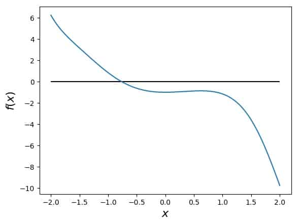
\(f(x)\) is represented by the blue curve. The black line is zero.
Note: I use python and mathplotlib to create these figures. I’ve pasted code examples below, together with those for the Netwon-Raphson method itself.
So how does this help? First of all, we can see what the function looks like. We can also see that it seems to have one root. Judging from the asymptotic behavior of both the sine and the cubic part, we can say right away that this is likely the only root of our function.
Furthermore, we see that this root lies somewhere between \(-1\) and \(-0.5\), but the exact numerical value of this root is hard to read off the graph. Still, that is already good enough for starting Newton’s method to find a more accurate value for the solution. We have seen a zero and we know more or less where it is.
Before we continue, a word of caution: when the function is not obviously well-behaved like it is in our example, visual inspection may actually be misleading. Unfortunately, I’ve seen even some of my fellow scientists argue something based on a graph, which would have needed some kind of backup or proof. In our case, we know that things are fine, because we know the functional form of \(f(x)\) and how its parts behave. So, if that is not the case, proceed with caution.
Finding the starting point \(x_0\) for the Newton-Raphson method
In our example, we can conveniently plot our function, look at the graph and pick a value for \(x_0\). However, that can be much more difficult in practice. So, what is important for getting a good first value for \(x_0\)?
First of all, it should be close to the actual root. Being close to the root helps, because in general that is enough to make sure that the method converges to a good result. As we’ll see below, strange things can happen, if \(x_0\) is chosen badly.
But if it is not easy to get a good enough plot of \(f\), for example because each value of this function is computed numerically and takes two days to produce, then one can just use any value as a starting point. Just have some argument ready as to why you expect your function to be well-behaved. Or, have an idea/estimate for your function in terms of what it should do and where.
In our example, knowing what happens during the Newton-method iteration, I suggest we use \(x_0=-1.5\) for quick and easy success. On the other hand, \(x_0=+1\) would not be such a good idea. Here are these two points marked on the graph of our function as red stars:
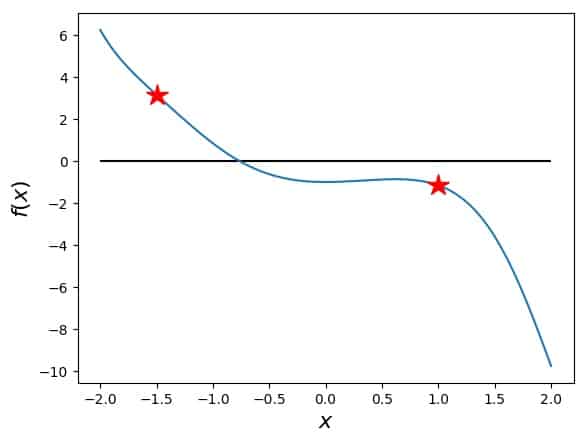
Why one of them works better than the other, and why proximity to the actual zero matters will be clearer in the following step. If you need more help on how to find good starting values for Newton’s method, please read my article How to Find the Initial Guess in Newton’s Method.
Constructing the tangent to the function for the next Newton-method step
This is the most complicated step of the whole procedure. But actually, it isn’t very complicated at all. If you had a ruler and a pencil, you could do it for both points on the figure above within a couple of seconds. So what do we have to do in terms of numerics?
The construction we are looking for is a linear function \(y(x)\) that touches our function \(f(x)\) at the point \(x_0\) and has exactly the same slope that \(f(x)\) has at the point \(x_0\). Denoting the derivative of \(f(x)\) with respect to the variable \(x\) by a prime, we can write this slope as
\[f'(x_0)\]Now, any linear function can be written in the usual form
\[y(x)=k x+d\]
where \(k\) and \(d\) are constants/parameters. Because we want \(y(x)\) such that its slope is the same as \(f'(x_0)\), we immediately know that
\[k = f'(x_0)\]
And because we also want the functions to be equal at \(x_0\), we know that \(y(x_0)=f(x_0)\) and so
\[k x_0+d =f(x_0)\quad\rightarrow\quad d=f(x_0)-k x_0=f(x_0)-f'(x_0) x_0 \]
So, with this information, we can go ahead and plot the tangent to our function at the point \(x_0\), if we know the values \(f(x_0)\) and \(f'(x_0)\). But how do we compute the derivative of our function?
To be honest, that depends on how you know your function. In our case, it is simple in the sense that we know the functional form of \(f(x)\) in a way that we can formally calculate the derivative. But in general, there is nothing wrong with, e.g., using a numerical derivative instead. Let’s keep it simple, though. Taking the derivative according to the rules of analysis, we get
\[f'(x)=2x \cos (x^2)-3x^2\]Using this formula, we can compute and plot any tangent to our curve (i.e., the tangent at any point on our curve). Here is our function again with the two points and the corresponding tangents:
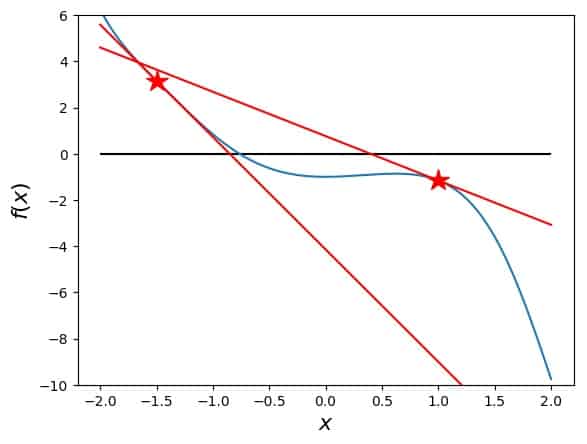
The tangents now show us the next step: finding their intersection with zero. In our case, one can see that one of them (for the left point at \(-1.5\) comes closer to the actual zero than the other). Still, this is not the only reason for the left point being the better starting value. The next iteration will already show us why that is, but before we get there, we need to calculate the successor to \(x_0\), \(x_1\).
Intersecting the tangent with zero to find the next step in the Newton-method
The intersection of a linear function with zero is straightforward to calculate. Given that
\[y(x)=k x+d\]
all we need to do is set \(y=0\) and get
\[0=k x+d\]
meaning that we find the successor the \(x_0\), by substituting from above for \(k\) and \(d\), as the solution to the equation
\[0= f'(x_0) x+f(x_0)-f'(x_0) x_0\]
which is
\[x_1= x_0 – \frac{f(x_0)}{f'(x_0)} \]
Note that we need \(f'(x_0)\ne 0\) in order for this to work. If \(f'(x_0) = 0\), we get a division by zero, which is a bad idea, both numerically and analytically.
Let’s plot these points in the figure for our example curve. The points are now visible on the zero axis, but not yet on the curve (that is the starting point of the next iteration step). So here we go:
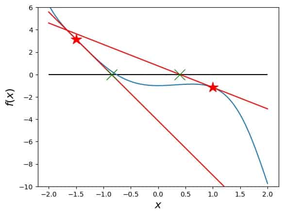
At this point, we have come from our first guess, \(x_0\) to our second one, \(x_1\). The basic idea of Newton’s method is, to repeat these steps until we approach the actual zero of our function enough, and the \(x_i\) do not change any more with a certain precision. At each step \(i\), we have:
\[x_{i+1}= x_i – \frac{f(x_i)}{f'(x_i)} \]
Repeating the tangent construction for Newton’s method
So, at this point, we repeat what we just did, but starting at \(x_1\) instead of \(x_0\). First, I added all steps (in green) to the figure, and here the new tangents at each \(x_1\) are for both our test starting point variants for \(x_0\):
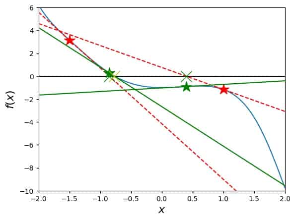
Now, this already looks somewhat messy, although I reduced the first (red) tangents to dashed lines. What we observe is that the green tangent on the left side, the one originating from the \(x_0=-1.5\) version of the iteration, has changed only a little from its red predecessor. The other green tangent, however, which comes from \(x_0=1\), is strongly tilted compared to its red predecessor, and is now actually pointing outside the figure.
This is a result of the function \(f\) running almost parallel to the horizontal axis at \(x_1\) for this alternative starting point. Following this weakly ascending line, we would find our next candidate for the root of our function well outside the region of interest. It is unclear that this would lead to any kind of success. Quite the contrary, in fact. This is a typical example for a failure of the Newton-Raphson method, due to a bad choice of the initial guess.
To be honest, my whole point of including this second initial guess was to show exactly that. Now that this is accomplished, I’ll replot the figure, but only with the left starting point and more zoomed in. In this way, the procedure is visible much more clearly:
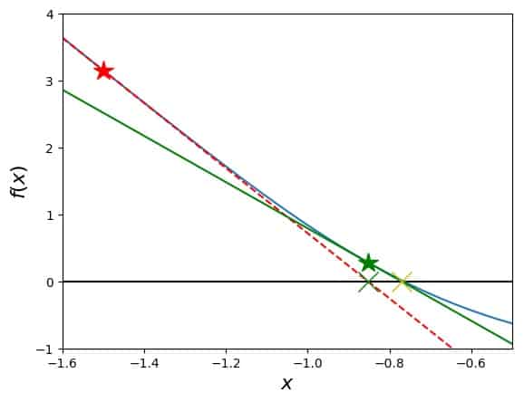
The starting value on the curve (red star) leads to the red tangent, down to zero (green X), back up to the curve (green star). The green star leads to the green tangent, down to zero at the yellow X, which is already pretty close to the zero of the blue curve, the graph of the function \(f\).
Waiting for convergence in the Newton-Raphson method
This iteration produces one value after the other, a so-called sequence of the \(x_i\) with \(i=0,1,2,\ldots \). Looking at these, we can decide whether or not Newton’s method has successfully produced an approximation to the root of the function under investigation. Let’s look at what happens for our example. The table below contains the value of \(i\), \(x_i\), the distance from the previous value, i.e., \(|x_i-x_{i-1}|\), and the relative change, i.e., \(|x_i-x_{i-1}|/|x_{i-1}|\).
| \(i\) | \(x_i\) | \(|x_i-x_{i-1}|\) | \(|x_i-x_{i-1}|/|x_{i-1}|\) |
|---|---|---|---|
| 1 | -0.851950113965 | 0.648049886035 | 0.432033257356 |
| 2 | -0.770224149559 | 0.081725964407 | 0.095928110187 |
| 3 | -0.764994622300 | 0.005229527258 | 0.006789617362 |
| 4 | -0.764972260820 | 0.000022361480 | 0.000029230899 |
| 5 | -0.764972260411 | 0.000000000409 | 0.000000000535 |
| 6 | -0.764972260411 | 0.000000000000 | 0.000000000000 |
Apparently, the value of \(x_i\) doesn’t change very much any more after \(i=5\), and both the absolute and the relative difference keep getting smaller. The latter is the better measure, because we could be watching a small number change by a small number, which would not necessarily be a small change in relative terms.
Naively, and in this case actually, this table means that we have a converged result and can stop the iteration. In practice, a certain small value is set for the desired precision, and as soon as the difference in \(x_i\) from one step to the next falls below this threshold, we declare the search a success and use the last \(x_i\) as the desired result.
And, we can now confidently declare that the solution of the equation
\[\sin (x^2)-x^3=1\]is \(x=-0.7649723\), if rounded to eight digits.
Convergence in the Newton-Raphson method for different initial guesses
It is interesting to ask whether we can always achieve a converged result with Newton’s method, no matter which initial guess we make, if we only wait long enough. Was it premature or just impatient of me to discard that other initial value, just because it didn’t look promising right away?
Let’s find out. I let the Newton-Raphson iteration run again with the initial guess \(x_0=1\), and here is the result. It takes a while, but actually, the iterations manage to find the correct solution as well:
| \(i\) | \(x_i\) | \(|x_i-x_{i-1}|\) | \(|x_i-x_{i-1}|/|x_{i-1}|\) |
|---|---|---|---|
| 1 | 0.396409399399 | 0.603590600601 | 0.603590600601 |
| 2 | 3.303061621796 | 2.906652222397 | 7.332450307184 |
| 3 | 2.160704263389 | 1.142357358408 | 0.345848031072 |
| 4 | 1.309230226393 | 0.851474036996 | 0.394072456570 |
| 5 | 0.900544139433 | 0.408686086960 | 0.312157540149 |
| 6 | 0.057382721002 | 0.843161418431 | 0.936279946213 |
| 7 | 9.561906891570 | 9.504524170567 | 165.633905199249 |
| 8 | 6.567704071213 | 2.994202820357 | 0.313138671429 |
| 9 | 4.206313448585 | 2.361390622628 | 0.359545831698 |
| 10 | 2.670109414753 | 1.536204033832 | 0.365213874955 |
| 11 | 1.589517654915 | 1.080591759838 | 0.404699430618 |
| 12 | 1.153299738573 | 0.436217916342 | 0.274434143586 |
| 13 | 0.699048420222 | 0.454251318351 | 0.393870997416 |
| 14 | -3.067625223777 | 3.766673643998 | 5.388287184460 |
| 15 | -1.805797626601 | 1.261827597175 | 0.411336948006 |
| 16 | -1.036124841598 | 0.769672785004 | 0.426223167904 |
| 17 | -0.800627833636 | 0.235497007961 | 0.227286325457 |
| 18 | -0.765944978892 | 0.034682854744 | 0.043319571575 |
| 19 | -0.764973033813 | 0.000971945079 | 0.001268948953 |
| 20 | -0.764972260411 | 0.000000773402 | 0.000001011018 |
| 21 | -0.764972260411 | 0.000000000000 | 0.000000000001 |
| 22 | -0.764972260411 | 0.000000000000 | 0.000000000000 |
This must be taken with a huge portion of caution, though. First of all, there is only one solution of the equation in our example. If there are more than one roots, Newton’s method can easily jump over to a different root, if the initial value is not chosen carefully. That means, it may not find different solutions at all. But back to the question we asked at the beginning of this section: what about yet another starting point? Let’s illustrate this some more.
Does Newton’s method always converge?
No. Newton’s method can fail to converge by reaching a point on the curve with zero derivative, by oscillating between two or more regions on the curve, by running off towards an asymptotic region, or if the function rises more slowly than a square root around the root. If the function doesn’t have any roots, Newton’s method must fail.
In my article Highly Instructive Examples for the Newton Raphson Method I show you concrete examples for all of this, so head over there, if you’d like to see the method fail for one reason or another. But for this article, I’d like to kind of summarize what can happen, which is presented next:
Let’s illustrate this by the following idea: we take our example function and investigate the number of steps it takes for Newton’s method to converge to the only root this function has. We’ll do this for all \(x\) as starting points \(x_0\), and plot the number of iterations needed as a new function \(g(x)\).
Ready? Here is the result:
A number of remarks about this figure are in order:
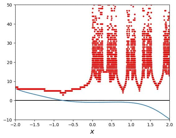
- The curve in blue is still our function from above, for comparison, and in order to see what its derivative is doing.
- The 10 000 points in red represent \(g(x)\) and are distributed evenly along the \(x\) axis.
- The function values of \(g(x)\) are discrete, because they can only assume integers. We are counting the number of steps needed for Newton’s algorithm to reach a desired relative precision of \(10^{-10}\).
So what can we learn from this figure? Well, the way it looks, the “left half” of the figure is much more suitable for starting points \(x_0\) than the “right half”. More precisely, negative starting values perform better than positive ones. Why is that?
If our starting position is to the left of the root, like our “good” example \(x_0=-1.5\), then the tangent in each step gets the next \(x_i\) closer to the root than the one before it was. As a result, a small number of steps is needed for the Newton-Raphson method to arrive at a converged result.
If, on the other hand, our starting position is to the right of the root, the function’s behavior and in particular the behavior of its first derivative are such that a lot of times, the next \(x_i\) is farther away from the root than the previous approximation. This is true, in particular, when the slope of \(f(x)\) becomes very flat, i.e., the value of \(f'(x_i)\) becomes very small, since that makes the difference between the \(x_i\) large. This is evident, when remembering the iteration procedure:
\[x_{i+1}= x_i – \frac{f(x_i)}{f'(x_i)} \]
The value \(f'(x_i)\) appears in the denominator, thus increasing the second term on the right-hand side of the equation, when \(f'(x_i)\) itself is small.
Regions of instability for the Newton-Raphson method
In the figure above, there are several “towers” of red points. What that means is that Newton’s method needed many steps for this method to converge, when it was started from a point around there. Equally well, this happens, if at some point during the iteration, the \(x_i\) happens to fall into this region, because that is the same situation like if the iteration had been started there.
These “towers” represent regions of instability for the Newton-Raphson method on the \(x\) axis. How can we understand those? Ok, we have seen that the first derivative of \(f(x)\), \(f'(x)\), is responsible for large jumps in the sequence of the \(x_i\). Let’s look at the first derivative of our example function. For
\[f(x)=\sin (x^2)-x^3-1\]we have
\[f'(x)=2x\cos (x^2)-3x^2\]The function \(f(x)\) has points with zero slope, where \(f'(x)=0\) . We can see immediately that \(x=0\) satisfies this equation, so there is one point to avoid. The other one is where
\[2\cos (x^2)=3x\]So, around each of those points, Newton’s method can be expected to not function properly, be thrown off far away from the root, or even hit one of these points. If the algorithm lands on one of these points precisely enough to produce a numerical value of zero for the derivative of \(f\), then the algorithm cannot continue.
However, in general it is unlikely to hit the exact numerical value of such a singularity with a grid point, unless that numerical value falls into some sort of pattern that the grid has, like being an integer, and the grid points are all integers. In our example this could happen for \(x=0\), but not likely for the other value.
Now, let’s discuss the plot from above a little further – I show it again here for your convenience:
Following the red curve from left to right, the first two towers of red points correspond to the two regions of instability that we just discussed, around \(x=0\) and \(x=2/3\cos (x^2)\). The following towers to the right are generated by starting points, whose first, second, third, etc. step falls right into one of these two regions of instability.
In between these towers of red points, we have the opposite, namely smaller regions, from which the first, second, third, etc. steps in the iteration takes the algorithm very close to the root, where it converges rapidly.
As I’ve mentioned above, the example function here has only one root, which helps the Newton-Raphson method to succeed. In this particular example, the only thing that can go wrong is the derivative hitting zero. There can be no on-going oscillation between regions or runaway towards an asymptotic region. So, our example here was made to show Newton’s method working well. For an investigation of the other possible failures, I refer you to my article Highly Instructive Examples for the Newton Raphson Method.
Before we get to the python code examples, let me summarize the algorithm for the Newton-Raphson method once again in compact form:
Summary: the algorithm for Newton’s method
The algorithm for Newton’s method for numerically approximating a root of a function can be summarized as follows:
- Given a function \(f(x)\) of a variable \(x\) and a way to compute both \(f(x_i)\) and its derivative \(f'(x_i)\) at a given point \(x_i\).
- Set values for the desired numerical relative precision \(\Delta_{d}\) of the result as well as for the maximum number of iterations \(N\) the algorithm is allowed to take.
- Choose an initial guess \(x_0\), ideally close to the location of the root to be approximated.
- Compute the next approximation \(x_1\) for the root as
\(x_{1}= x_0 – \frac{f(x_0)}{f'(x_0)} \). - Repeat as \(x_{i+1}= x_i – \frac{f(x_i)}{f'(x_i)} \) and compute the relative difference between the approximations as
\(\Delta= \frac{|x_{i+1} -x_i|}{|x_i|}=\frac{|f(x_i)|}{|f'(x_i)x_i|} \),
until one of two things happens:- the maximum number of allowed iterations is reached, i.e., \(i>N\)
- the desired numerical relative precision is reached, i.e., \(\Delta<\Delta_{d}\)
If the algorithm reaches the maximum number of iterations that you set, this can but does not have to indicate that convergence is not possible. Experimentation with suitable values for both \(\Delta_{d}\) and \(N\) may be needed to arrive at a satisfactory result.
Using Newton’s method without a computer
This is interesting to mention, because it does not automatically come to mind when I think about computational algorithms: you can do all that I just described by hand, i.e., with a pencil and paper.
I’d probably skip detailed plotting of the function and only sketch its graph. I’d also make sure that I choose an ideal starting point and not fool around too much. But other than that, the steps are the same.
For this to work by hand, the functional form of \(f\) must be known and you need to be able to evaluate the function and its derivative reasonably accurately. Otherwise, the precision that you can achieve in your root-finding efforts will suffer. And don’t make a mistake when calculating. And … you get the picture.
If you’d like to see an application of Newton’s method could be and actually is used to get results, I refer you to my article Highly Instructive Examples for the Newton Raphson Method. The first example there shows you how to calculate the square root of a positive real number with Newton’s method. Have fun!
Python code for creating the figures
As promised, I post my python code for this description and the example here. First, I post the entire code I have used to generate all the different figures in this article. Please note that this code isn’t perfect, it is just an example. Furthermore, the code comes as is and without warranty or anything like that. Also: use the code at your own risk.
As I have several different steps and figures in this article, I could post several pieces of code here. However, I have decided to post only one code piece here for the figures, and only separate out the part for the Newton-Raphson algorithm below by itself.
Various lines in this code are commented out, but that only means that you can switch around between different settings to produce one figure or the other. Don’t worry, it isn’t very complicated.
#!/usr/bin/env python3
# -*- coding: utf-8 -*-
"""
Created on Tue Sep 24 05:52:47 2019

@author: Andreas Krassnigg, ComputingSkillSet.com/about/

This work is licensed under a
Creative Commons Attribution-ShareAlike 4.0 International License.
More information: https://creativecommons.org/licenses/by-sa/4.0/

"""

import matplotlib.pyplot as plt
import numpy as np

# define the function to investigate
def f(x):
    return np.sin(x**2) - x**3 - 1

# and its derivative
def fp(x):
    return 2*x*np.cos(x**2) - 3*x**2

# define left and right boundaries for plotting

# for demo reasons:
interval_left = -2
interval_right = 2

# for better search:
#interval_left = -1.6
#interval_right = -0.5

# define x grid of points for computation and plotting the function
# increase num at your convenience, but with caution. Article figure has 10 000
xvals = np.linspace(interval_left, interval_right, num=100)
# define y values for example function
yvals = f(xvals)

# create a list of startin points for Newton's method to loop over later in the code
# demo list of starting points
#pointlist = [-1.5,1]
# good starting point
#pointlist = [-1.5]
# not so good starting point
#pointlist = [1]
# try all x values as starting points
pointlist = xvals

# begin figure for plotting
plt.figure()

# plot the function f
plt.plot(xvals,yvals)

# plot the zero line for easy reference
plt.hlines(0, interval_left, interval_right)

#label the axes
plt.xlabel("$x$", fontsize=16)
plt.ylabel("$f(x)$", fontsize=16)

# set limits for the x and y axes in the figure
# set x limits
plt.xlim((interval_left, interval_right))
# set y limits
# for demo reasons:
#plt.ylim((-10,6))
# for better search:
#plt.ylim((-1,4))
# for convergence plot:
plt.ylim((-10,50))


# loop over all starting points defined in pointlist
for x0 in pointlist:
    # set desired precision and max number of iterations
    prec_goal = 1.e-10
    nmax = 1000
    # initialize values for iteration loop
    reldiff = 1
    xi = x0
    counter = 0
    # start iteration loop
    while reldiff > prec_goal and counter < nmax:

#        # plot the tangents, points and intersections for finding the next xi
#        # plot star on the curve where x=xi
#        plt.plot(xi,f(xi),'r*', markersize=16)
#        # compute y values for tangent plotting
#        tangy = fp(xi)*xvals + f(xi) - fp(xi)*xi
#        # plot the tangent
#        plt.plot(xvals, tangy, 'r--')
#        # perfom iteration step and compute next xi
#        x1 = xi - f(xi)/fp(xi)
#        # print numbers for use in convergence tables (csv format)
#        print('%i, %15.12f, %15.12f, %15.12f' % (counter+1, x1, np.abs(f(xi)/fp(xi)), np.abs(f(xi)/fp(xi)/xi)))
#        # plot next xi on the axis
#        plt.plot(x1,0,'gx', markersize=16)
#        # trade value to next iteration step
#        xi = x1


        # get the number of necessary iterations at that particular x0
        # compute relative difference
        reldiff = np.abs(f(xi)/fp(xi)/xi)
        # compute next xi
        x1 = xi - f(xi)/fp(xi)
        # trade output to input for next iteration step
        xi = x1
        # increase counter
        counter += 1

    # plot the number of necessary iterations at that particular x0
    plt.plot(x0,counter,'r.', markersize=5)
    # print test output
    print(x0,counter,reldiff)

# save the figure to an output file
plt.savefig('newton-method-demo-figure.jpg', bbox_inches='tight')

# close plot for suppressing the figure output at runtime. Figure is still saved to file
#plt.close()
Python example code for the Newton-Raphson method
In this section, finally, I post a short code snippet in python 3 for computing an approximation to a root of a function numerically with the Newton-Raphson method. Replace the function and its derivative by the one you want to investigate. Set a starting value, a desired precision, and a maximum number of iterations.
#!/usr/bin/env python3
# -*- coding: utf-8 -*-
"""
Created on Wed Sep 25 11:16:33 2019

@author: Andreas Krassnigg, ComputingSkillSet.com/about/

This work is licensed under a
Creative Commons Attribution-ShareAlike 4.0 International License.
More information: https://creativecommons.org/licenses/by-sa/4.0/

"""

import numpy as np

# define the function to investigate
def f(x):
    return np.sin(x**2) - x**3 - 1

# and its derivative
def fp(x):
    return 2*x*np.cos(x**2) - 3*x**2


# set initial guess
x0 = -1.5

# set desired precision and max number of iterations
prec_goal = 1.e-10
nmax = 1000

# initialize values for iteration loop
reldiff = 1
xi = x0
counter = 0
# start iteration loop
while reldiff > prec_goal and counter < nmax:
    # get the number of necessary iterations at that particular x0
    # compute relative difference
    reldiff = np.abs(f(xi)/fp(xi)/xi)
    # compute next xi
    x1 = xi - f(xi)/fp(xi)
    # print progress data
    print('%i, %15.12f, %15.12f, %15.12f' % (counter+1, x1, np.abs(f(xi)/fp(xi)), reldiff))
    # trade output to input for next iteration step
    xi = x1
    # increase counter
    counter += 1
Further information on the Newton-Raphson method
Here on ComputingSkillSet.com, I have written other articles on Newton’s method. One, Highly Instructive Examples for the Newton Raphson Method, is about concrete examples that show you some of the features that I could only mention in the present article. Another, How to Find the Initial Guess in Newton’s Method, shows you how you may find a suitable initial guess for your Newton-method problem at hand. Yet another, Newton Fractals Explained: Examples and Python Code, shows you an impressive extension of this method to complex starting values.
Fun reading on the Newton-Raphson method
While the Newton-Raphson method can seem like very serious business at times, it is equally important to have some fun explaining it. If you are in for a try, read one of these: