Martingale Roulette Strategy: Full Outcome Analysis with Charts

Does the Martingale Strategy work for Roulette? Well, that depends on what you mean by work. Will you win? How much? When? Will you lose? How much? When? I have asked myself all of those questions and ended up writing a bit of Python code to find the answers, with the help of Monte Carlo Simulation.

The Martingale system has a high winning probability in the short term, but the probability for a total loss rises strongly in the long term. The table maximum plays an important role in reducing the probabilities of a total loss, but also of winning overall.

Martingale Roulette Strategy: Full Outcome Analysis with Charts

Now, how was I able to figure all this out? How can one find such statements in the first place? I’ll explain all of this below, but even better: I’ll show you a couple of cool charts and detailed overview tables that will help you understand what’s going on, when the Martingale System is used in Roulette.

At this point, I strongly urge you to take a look at my simulation disclaimer. After you have read the simulation disclaimer, you’ll know better (I hope) what to make of the information contained in this article and what not to conclude from it.

Here you'll learn more about:

What is the Martingale Strategy?

The Martingale strategy in general refers to the following idea: When someone is betting on some game outcome with two possibilities with roughly equal probability, one uses the following betting system:

start with a certain base amount, say 10 $, bet this amount in the first round
if you lose in this round, double the amount you just lost and bet that double amount in the following round. If you just lost 10 $, now you bet 20 $.
if you lose again, double the amount again for the next round. In our example, if you just lost 20 $, you now bet 40 $.
if you win, you reset the amount for the next round back to the base amount, in our example 10$.
this kind of system is often called a progression.

Here is a graph of what that progression looks like:

The point is that each win gives you back all of what you lost in that particular batch of rounds from the base amount up to what you had to bet in order to win. Doesn’t sound convincing?

Indeed, there is a catch: If you lose often enough in a row, all your money will be gone very quickly. The reason is that the betting amount increases exponentially with the number of losses in a row. Sounds complicated? Somewhat, but let me add one more piece of information before I start explaining: the basic odds for an immediate total loss.

Probabilities for a Single Progression in the Martingale System

There is one interesting piece of the Martingale puzzle that I want to show you before I’ll start putting it all together for you: the probabilities for having subsequent losses for a certain number of rounds in a row.

Let’s assume for simplicity that we are dealing with a fair and even chance of winning: 50/50. I know that’s not quite the case for the application to Roulette, which we’ll discuss below, but the difference is not important for our argument (see also below, where I talk about the house edge).

So the probability to lose a single bet or round is 50/50, in other words, one half:

\[p_1 = 1/2\]

For two subsequent rows, the probabilities of two individual rounds are combined by multiplication, since the two rounds’ outcomes are completely independent. So we find

\[p_2 = 1/2\;1/2 = 1/4 = \frac{1}{2^2}\]

For more than two rounds we can simply generalize this (because it is easy to see that this formula is correct) to

\[p_n = \frac{1}{2^n}\]

With more rounds in a row, we see that losing all of them becomes less likely, but the probability for a total loss right from the start in the first (and in such a case only) progression is always non-zero. Which means that you can lose all your money with a certain, albeit small, probability at all times while you use this system. How probable at what time? I’ll show you below. But that was quite a bit of theory wasn’t it?

Right, we could really use a table to understand this better, so here we go:

Overview Table of Amounts and Simple Probabilities for a Martingale Doubling-Up Strategy

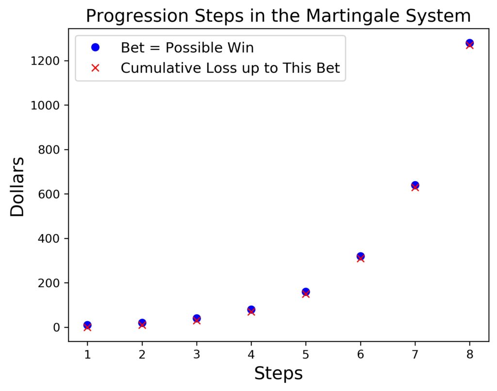
The following table shows you the progression details for the doubling-up of bets, which equal the possible win in each round, collective losses, and probabilities for a losing-all-streak for a number of steps up to 12. We start with a base amount of 10 $.

Step	Bet = Possible Win	Cumulative Loss up to this bet	Probability for total loss after n steps for 50/50 chance in percent, rounded
1	10	0	50
2	20	10	25
3	40	30	12.5
4	80	70	6.25
5	160	150	3.13
6	320	310	1.56
7	640	630	0.78
8	1280	1270	0.39
9	2560	2550	0.20
10	5120	5110	0.10
11	10240	10230	0.05
12	20480	20470	0.024

Now what does all that mean? It basically means a number of things:

As soon as you win, you only win the base amount over what you have already lost before, in our example 10 $. You can easily see that by comparing the second and third columns in the table. Why?
Because doubling up after a loss makes both the bet and the possible win exponentially higher with every round. However, that has to compensate for the sum of all the individual lower bets that you will have placed (and lost) before you eventually win.
Depending on how much money you have, you can quickly see how many steps in this scheme you are able to follow through with. If you have 1270 $ to start with, for example, you can double up to step seven.
If you lose enough times in a row right from the start, that means game over as soon as you reach your starting amount of money that you bring to the table.
The probability for a streak of n losses in a row gets smaller exponentially as well. However, we’ll keep a close eye on those lower numbers of n, because we’ll see that you cannot, in practice, go up arbitrarily high in the progression (and not just because you run out of money).
Example: Let’s say, 100 gamblers show up with a starting amount of 150 $ each. That means, they can go up to step four in their first progression. The probabilities tell us that, on average, 6 of the 100 can go back home empty handed right after the first four rounds.
One more example: Let’s say, 1000 gamblers show up with a whopping 10000 $ each (plus some change, actually). That means they could go all the way up to step 10 in the progression, if necessary. Still, on average, one of them will have lost all of their money right after the first 10 rounds.
The losses outweigh the wins: we’ll see further down in nice graphs and more, how much one can win with this strategy after how many rounds and with what probability. But one thing is easy to see already at this point: We have seen how quickly you can lose all your money after only a couple of rounds. But how much could you win during the same number of rounds in the ideal case, when you win every time? The number of rounds times the base amount.
Yes, in our example that means a mere 40 $ after four rounds, or 100 $ after ten rounds. But that unlikely maximum win stands against a possible complete loss of 1270 $ and 10230 $, respectively.

So all that doesn’t sound too promising, or does it? Let’s dig in deeper, and find out.

Does Martingale Work for Roulette?

Yes, the Martingale Strategy can be applied to Roulette, since there are betting possibilities in Roulette that offer almost even odds. Does it work in terms of will you win? Not with certainty, that should be clear by now. However, there are many interesting aspects of what works and what doesn’t. I’ll show you all the details further below.

Before that, let’s quickly explore the situation and useful bets at the Roulette table. In Roulette, there are various bets with different odds and, accordingly, different returns for what you bet, in case that you win.

The game is based on the spinning Roulette “wheel”, in which a ball is cast to roll around the wheel a couple of times before it drops in one of 37 or 38 (depending on the variant of Roulette) little boxes with the numbers from 1 to 36. The remaining box, or boxes for American Roulette, are 0 and 00.

Each number is assigned a color, either red or black, except for 0 and 00. In addition, each number is obviously odd or even, but again 0 and 00 are neither odd nor even. You can also place bets on individual numbers and various groups of numbers, but the odds for those bets are too far away from 50/50 to be useful.

For our analysis, let us therefore stick with the red-or-black bet as well as the odd-or-even bet. In both cases, the odds of winning are 18/37 (or 18/38 for American Roulette), the odds of losing are 19/37 (or 20/38 for American Roulette). The important thing here, however, is that in both these cases (kinds of bets), a win is equal to the amount that was bet. So if you bet 10 $ and win, you’ll get your bet back plus 10 $ in addition.

The small probability difference in disfavor of the player is called the house edge and I’ll discuss it below. However, this discussion will be brief, because its role is marginal for the topic of the Martingale strategy in Roulette, which is why I’ll just ignore it for now. The values of the probabilities need to be known; that is all we need for the simulation.

Steps in the Martingale Strategy for Roulette

In order to employ the Martingale Strategy for Roulette, you follow these steps:

You pick a type of bet that offers the win-what-you-bet return as described above
You bet the base amount (e.g. 10 $) in the first round on one of the outcomes.
It doesn’t matter which outcome you bet on. Just choose red or black, odd or even, as you like.
If you win, you bet the base amount again.
If you lose, you double your bet in the following round, i.e. 20 $ after one loss, 40 $ after two subsequent losses, etc. (see the table above)
As soon as you win after a couple of subsequent losses, you return to the base amount for the bet in the following round.

This steps are followed until one of the following things happens:

You keep losing subsequent rounds until you lose all your money
You decide to walk away

At the time you walk away, you’ll either have a net win or a net loss. Below, I show you graphs for probabilities of winning or losing as the number of rounds increases and you keep playing. But before that, there are a couple of other things that need clarification.

Are Streaks Important in the Martingale Strategy?

First of all, both winning and losing streaks are just illusions. Every spin of the roulette wheel is completely independent of all of the spins that came before it (and of all the spins that will come after it as well). It is useless to look for patterns in the numbers or the red/black pattern. It is a random pattern and cannot be predicted.

Anyone telling you otherwise is either lying to you or doesn’t know any better, neither of which are reasons to trust someone. Even if they try to convince you that there are devices that can reliably predict the numbers at the table shortly before rien ne va plus is called by somehow monitoring the ball and then calculating stuff, that’s not true. Devices like this are pure fiction.

The randomness argument leads to an important point: If you want to follow the Martingale strategy in Roulette, all you have to do is to always bet on something where the possible win equals the bet. In other words: it is not necessary to bet on red all the time. You can mix bets on red and black, even and odd in any way you want, and you’ll still follow the system.

There are no streaks. So you don’t need to follow one for Martingale, either.

Is the Martingale System Allowed in Casinos

Yes, the Martingale system is allowed in casinos in principle. But what does in principle mean? It means that you can place your bets according to the rules for that particular Roulette table in that particular casino.

Now what exactly does that mean? Well, it means that in a real casino there are rules and limits for bets that can be placed at a Roulette table. We can simulate an infinite amount of bets all we want (don’t worry, we’ll still do that and look at the most general case), but we’ll have to think about actual limits at actual Roulette tables in actual casinos when interpreting the results or even when configuring the simulation.

Let’s explore those limits for a bit, shall we?

Practical Restrictions to Using the Martingale Strategy for Roulette in a Casino

There are two main restrictions that the setup of a Roulette table in a real casino places on the Martingale strategy. One is the amount of rounds you can play in succession, the other are the table lower and upper betting limits. Let’s look at these, one after the other.

The restrictions imposed are the following:

The table minimum for outside bets (such as red versus black or odd versus even) determines how low your base amount can be.
The table maximum for outside bets determines how high you can actually go in the doubling-up progression (Wait, aaaaargh!)
The average time between spins of the Roulette wheel in a casino determines how many rounds you’ll be able to play in an hour.

On first glance, that last one sounds ok, but the other ones threaten to severely interfere with the Martingale system. Let’s check out what it means to have a table minimum and maximum:

The minimum determines how low you can start with your base amount. Basically, the whole progression system must fit in between the minimum and the maximum, so we better set our base amount to the table minimum.
The maximum determines how much money you can bet in a single round. Looking back at the table above, the problem is that the system grows exponentially. So there won’t be too many steps possible, unless the table maximum is rather high.

So where are we in real casinos? If I can trust what people write, it is reasonable to assume a table minimum of 5 $ or 10 $ for outside bets. The corresponding maximum seems to vary, depending on where you are (and what kind of table it is, but we’ll look at two typical values: 150 $ and 1000 $. In addition, we’ll also have the unlimited version of the simulation, which as an approximation corresponds to any very high limit (you’ll see soon, what kinds of differences different limits produce).

Ok, so starting at a base amount of 10 $, 4 steps in the Martingale progression lead up to the 150 $ limit, and 7 steps almost correspond to the 1000 $ limit (that’s close enough to 1270 $ for our purposes). Is that enough to get something out of the system?

The other practical restriction on playing Roulette in a casino is the average rate of spins of the Roulette wheel per hour, which is of the order of 40. So, if you play for one hour, you’ll be able to play 40 rounds, 200 rounds in 5 hours, and 10 hours of playing gives you 400 rounds. We’ll use these numbers as guides when we discuss the practical use of the Martingale system for Roulette in a casino below.

What is Monte Carlo Simulation and How Does it Help?

Monte Carlo simulation is a numerical computational technique that allows us to compute and simulate complex systems that are based on chance and other mechanics. The method is grounded in the usual simple arguments of probability, like the one I used above to provide the probabilities of total loss in a single progression of the Martingale system.

To describe comprehensively, how Monte Carlo simulation works, is beyond the scope of this article. The short version is: Monte Carlo simulation can in principle handle any level of complexity, which is in sharp contrast to a strict attempt to calculate probabilities based on trees for all possible outcomes in the system – there are simply too many.

The twist in Monte Carlo simulation used to make it feasible is to actually simulate a run through the system, and pick – at random – certain events during the run, for which the individual probabilities are known. Like in our case: we know the probabilities at each spin of the wheel, but it would be rather complicated to compute all variations that could happen with combinations of wins and losses in arbitrary succession.

In Monte Carlo simulation, we play out a game with well-defined rules by following the steps and picking at random the outcomes at every step, where such a random event occurs. Then we repeat the run, again and again, a lot of times. This way, we end up with a sample of possible runs and outcomes, which represent but approximate the entire set of possible outcomes. In the end, we can look at various numbers that summarize what happened and how often, which gives us an idea of what’s going to happen in the actual system that we simulated.

Importantly, the cool thing is that we can track all these interesting quantities and results through all stages of the run. This will become clearer in the next section, when I explain Monte Carlo simulation again, but for the particular case of Roulette.

Monte Carlo Simulation of Roulette

Say, we have a computer program that can take into account the probabilities in Roulette and execute a number of subsequent random events, where the player wins with the winning probability and loses with the losing probability. As mentioned above, for the win-what-you-bet cases, these are:

winning: 18/37 (or 18/38 for American Roulette)
losing: 19/37 (or 20/38 for American Roulette)

So the system can then simulate how playing Roulette will turn out for a player, if we tell it how much the player bets in each round. Once that is fixed, we can let the system run and observe what happens, like:

How many rounds does it take for the player to win at least 10 $?
How many rounds does it take for the player to lose all his money?
How probable is it that a player can walk away with a net win after 10 rounds?
How does this probability change with the number of rounds?
What is the average money in hand for a player after 40 rounds = an hour?
What about after 5 hours?
How does the average money in hand change over time?

All these are valid questions, and we can be really creative in the way we look at things. However, we have to be scientific about it, which means that we’ll take averages over large numbers of runs to minimize statistical fluctuation.

This is like looking at one thousand people playing Roulette and recording everything that happens to every single one of them. Sounds tedious, right? It is, but that’s done by the computer completely automatically in the program, because it just simulates people playing. How much we can do, simulate, and try out is just a matter of programming and letting the code run on powerful enough computers. The calculations for the present article, by the way, can be done on a laptop.

So, to lead over to our simulation results of the Martingale system for Roulette, I’ll give you one more concrete example for what happens in the Monte Carlo simulation: say, we did a thousand runs of playing Roulette with the Martingale for a specified number of rounds, which corresponds to a thousand people playing Roulette with the Martingale system. How many of those runs turned out to have zero money left after the given number of rounds? That gives us the probability that the average player will lose everything, if they play in the way we simulate.

Monte Carlo Analysis of the Martingale Strategy for Roulette

Monte Carlo analysis for Roulette needs the given probabilities for the possible events (the outcomes of a spin of the wheel) as well as some mechanism to determine a bet. Then it will generate a random number to determine the outcome of a spin, i.e. whether the player wins or loses in each round.

In the Martingale Strategy, we have the following rules programmed into the simulation:

The base amount of the progression (basically the table minimum, say 10 $)
The total funds available in the beginning, or, alternatively, the number of steps we want to be able to play doubling up each time. Depending on which one of these is given, the other can be deduced.
The probabilities for winning or losing (as given above)
The win and loss for a bet (equal amount win or total loss of bet in our case)
The amount to be bet in each round as:
- Base amount after a win
- Double the previous bet after a loss, unless
  - not enough funds left, then bet all that is left
  - table limit is reached, then bet the table limit
  - nothing is left, then bet zero (equivalent to game over)
Keep track of level in the progression
Keep track of total funds in hand

Each simulation is set up by using a certain number of samples, in my case 20, and a preset sample size, in my case 10000 runs. In total, the simulation will thus contain 200 000 runs each, which allows for reasonable statistics and, in particular, good enough (i.e. small enough) statistical errors.

The number of rounds is preset for each simulation. At the end, the numbers of net wins, net losses, total losses, and average funds in hand are computed in each sample and averaged over the samples. So this kind of setup is behind all the graphs you’ll be looking at below.

The Martingale Strategy for Roulette With no Table Maximum

Before we dive into the more practically relevant results involving table limits and the like, I’d like to show you a few graphs using the unlimited version of the Martingale strategy for Roulette. We’ll use these to get used to what’s on the graph, how to interpret the curves, and what to expect from a simulation like this.

The most burning question on you mind right now is perhaps: what does a simulation like that produce? What do the results look like? The best thing to show you first, in my humble opinion, is the following graph, which tracks the funds of 100 players through 40 rounds of following the Martingale strategy with a base amount of 10 $ and a 7-step-progression starting fund of 1270 $.

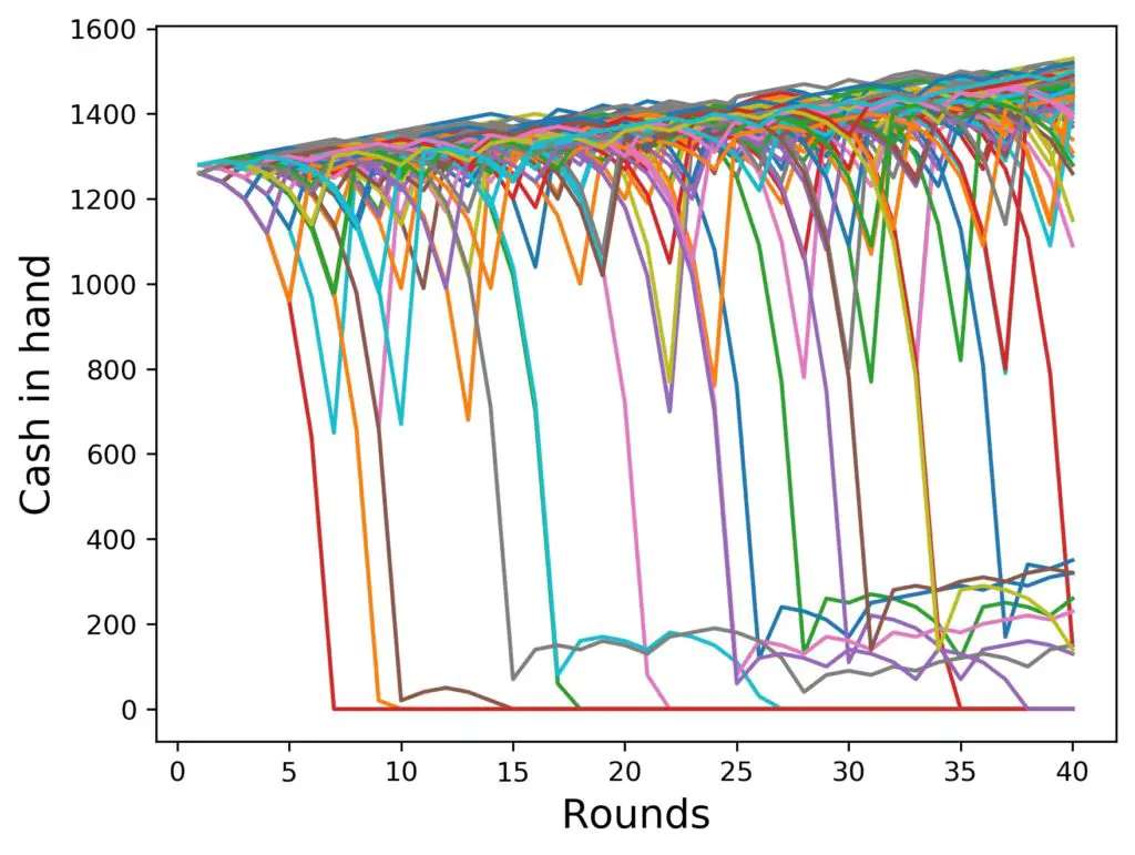
What are these curves? Each of the curves in different colors is the track of money in hand, that one of the 100 players in this graph has over time, plotted as a function of the number of rounds. I chose 40 rounds, because that amounts to roughly one hour of playing Roulette in a casino.

A few things to notice:

All curves start at round 1 and an amount of cash of 1270 $ plus or minus 10 $, depending on whether the first bet was lost or won.
After round 1, our rules apply. Whoever loses, doubles the bet, whoever wins, wins the same amount of 10 dollars net over the amount held before a possible preceding losing streak had begun.
We can see a couple of the curves nose-diving, one of them even right from the beginning.
Whichever curve hits zero, stays there.
If a recovery happens with a bet that’s been doubled up from the previous one, the curve goes back up roughly to where it was before.
If a recovery happens with a bet that could not match double the previous bet, because not enough funds were available, the curve continues to rise gradually again, but from a (substantially) smaller amount of cash in hand.
The majority of the curves seem to stay around the starting amount, at least on the scale of number of rounds that we are looking at here.

Sounds and looks interesting, doesn’t it? What about more players? Let’s look at the same figure, but with 1000 instead of 100 runs (= players):

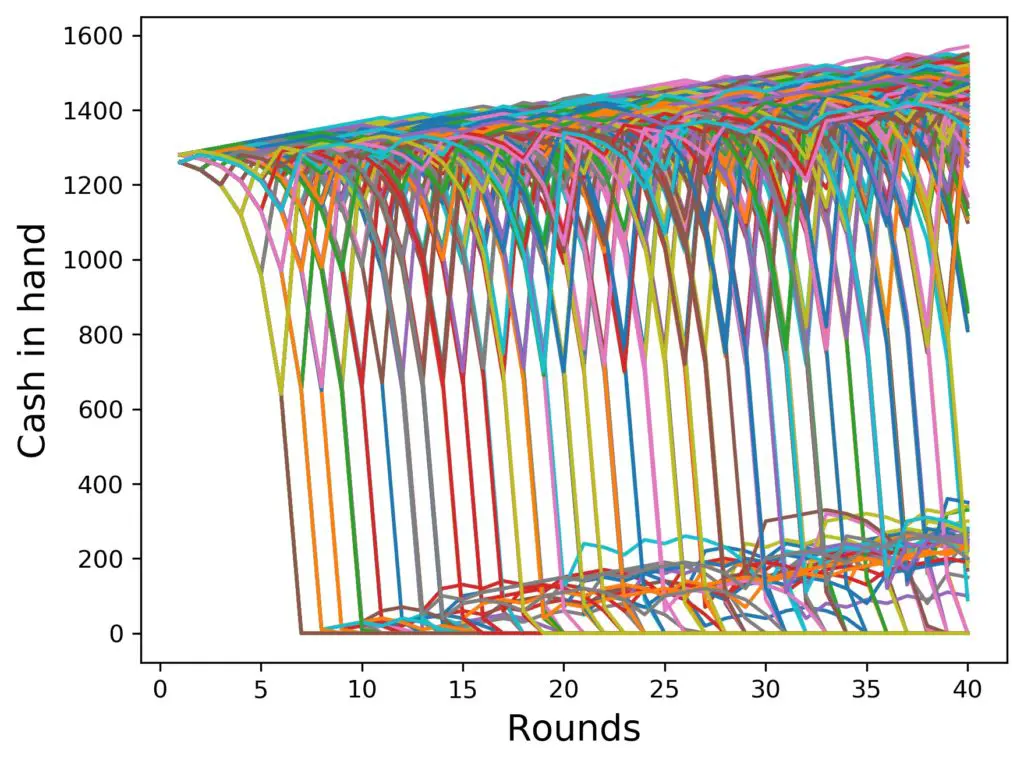
Here we can clearly see how the bottom region of the graph gets populated with unlucky players. Yes, there are more on top, too, the ratios are the same, just the statistics get better, if we use more. On the other hand, the graphs get somewhat full, if we use too many runs for these, so we’ll stick to 100 for the current series of graphs. Yes, there are more!

The next scope for this plot is one where we look at the development over 200 rounds, that is roughly five hours of playing Roulette in a casino. Showing you 100 players again in the same setup without limits, we get the following chart:

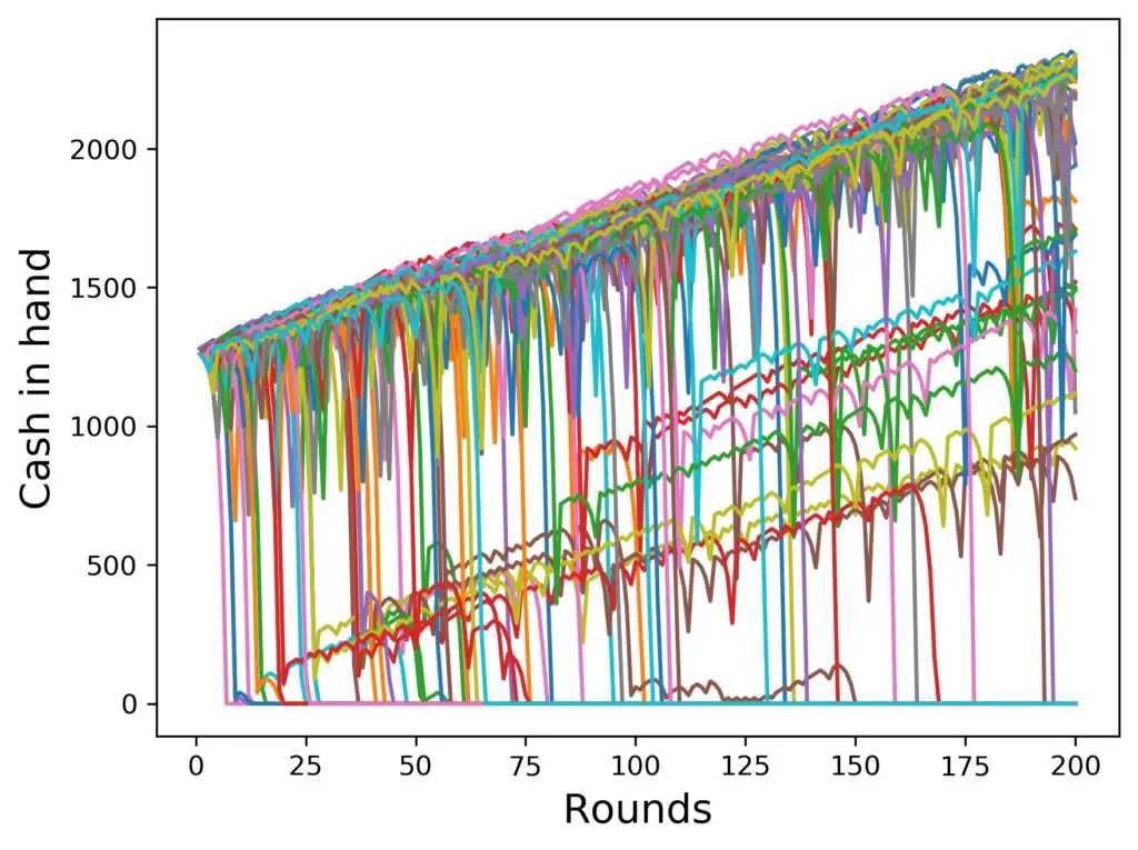
What’s new in this figure? Not too much, actually, except that there are a number of trajectories (curves) that are in the region between the bunch at the top and the flat bottom line of total loss. We can see that those come at any various heights.

This is a result of the following effect: if a player loses several times in a row after a while of winning, it happens that the amount left to bet is lower than the player would need to double up for the subsequent bet. Then, the simulation bets all that is left on the player’s behalf. If they lose, they land at zero anyway. But if they win, they cannot fully recover to where they were at, before the losing streak had begun. They just recover to the amount that was left to bet, which is somewhat lower than the bulk of recovering curves at the top of the chart.

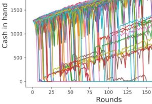
But does that behavior simply continue? How far can the top bunch keep winning and increasing their money in hand? Let’s find out by running the simulation further out. Here is what’s going on up to 400 rounds, which corresponds to about 10 hours of playing – maybe a long day at the office for a gambler:

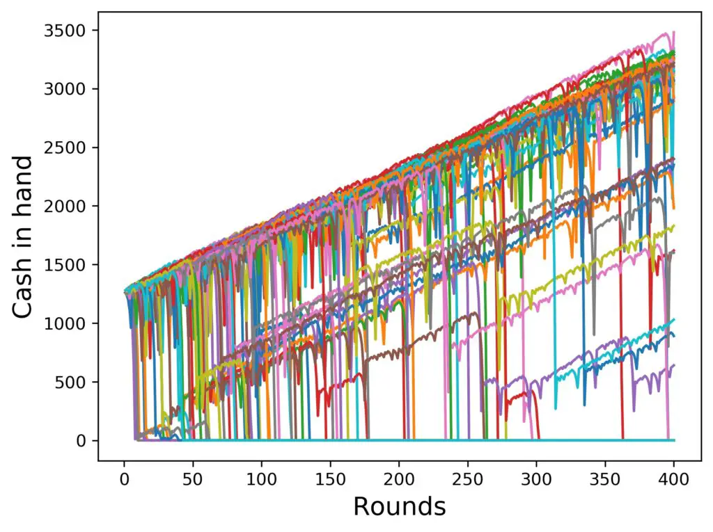
Here we notice the bulk at the top getting thinner towards the right of the chart. More and more players are dropping from the top. While the bottom line doesn’t look that spectacular, don’t be deceived by the single line – there are still many lines lying on top of each other at zero. One can see this best by observing all the curves that dive to zero over time. The only reason this looks like a single line is, that they lie on top of each other exactly, unlike the ones at the top of the figure.

But let us not stop there. Scaling up by a factor of 10, we arrive at 4000 rounds, i.e. 100 hours of playing. This sounds like a lot, but can certainly be done in successive sessions. All that’s needed is to remember which size of bet was placed last and to place the next bet accordingly in the next session at the table. Alright, 100 players playing for 4000 rounds:

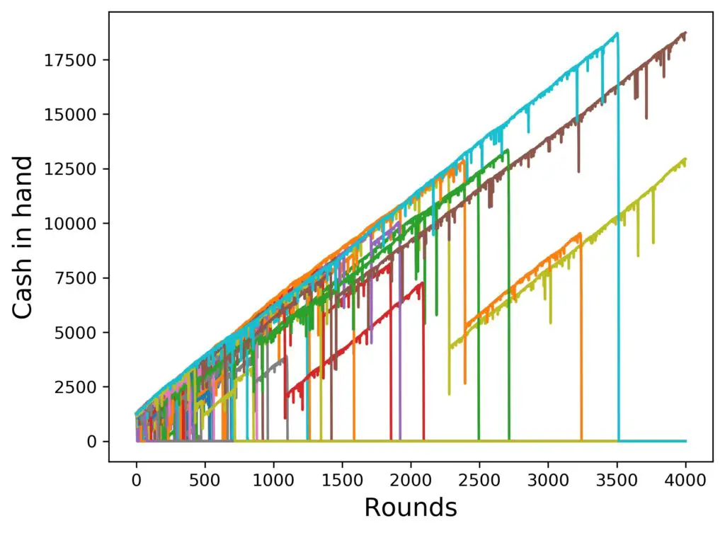
Aha! Finally, we see some clear development: Almost all of the 100 players drop to zero over the course of 4000 rounds! In this particular example, two of them are still alive and playing, and with substantial amounts of cash in their hands. All others (keep in mind, 98 percent in our example) have lost all their money!

That’s kinda bad, but just to show you that nothing lasts forever, here is a run with 100 players, that went up to ten times more rounds (even) than we’ve just seen: 40 000 rounds. The result: total elimination:

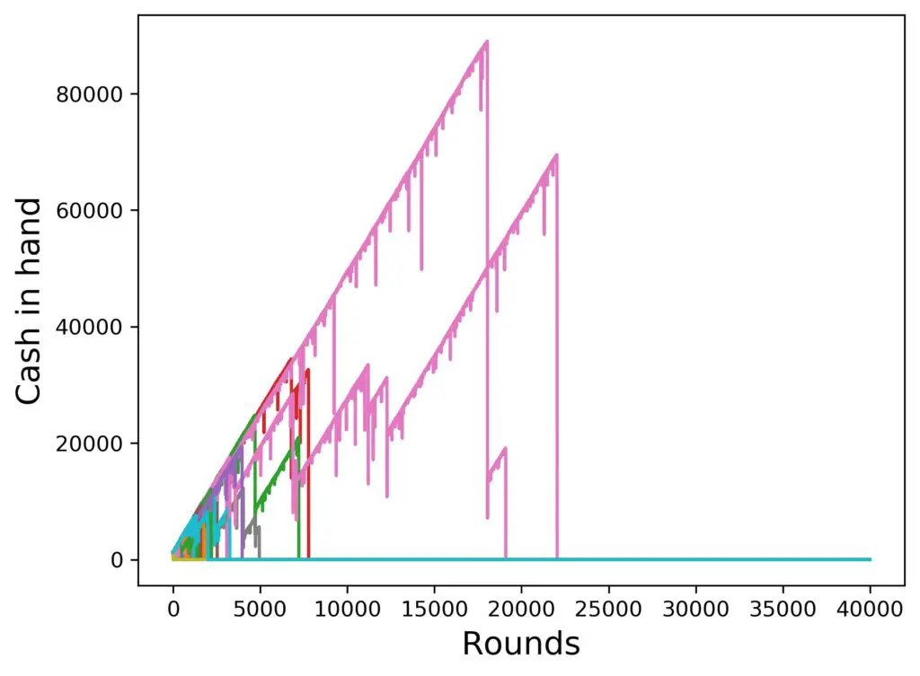
In this particular example, all players are out of money before they reach 25000 rounds. Granted – that corresponds to a long time playing, like 625 hours or 26 days non-stop, without ever sleeping or doing anything else. But hey, over time, you can certainly accumulate that sort of amount of playing rounds.

What are the important takeaways from this last two graphs? I would say this:

If we get to play the Martingale system in an unrestricted manner, a very small percentage of players can reach very high net wins (before they then lose everything in an instant). In this particular example, we had two players go beyond 60 000 $ from a starting amount of 1270 $.
The higher the funds in hand get, the longer the progression becomes. Looking at the table above, we see that steps up to 13 are possible in this range of money in hand.
Important: Although some players are extremely lucky and reach high amounts of cash, eventually, they all lose. In fact, this is inevitable, so don’t ever count on being able to keep winning forever!

You know what? Let’s increase the statistics of this very long runs a bit and step it up from 100 to 10 000 players. What can we expect from this? More densely populated areas on the graph and more extreme outliers. Alright, here we go – 10 000 players for 60 000 rounds:

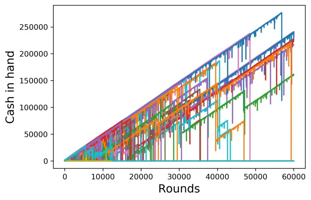
There are a couple of things that we see here:

More people play, the outliers get more extreme, indeed. Winnings of up to 250 000 $ before the drop, and a handful of players actually survive 60 000 rounds. But keep in mind, all the other 9995 players lost all their money, some very soon into the game.
We have not yet discussed the slope of those curves on the top. That looks nicely linear, and it actually is. But why and how much slope is there? Expecting an almost equal probability for winning and losing in each and every round, we’d expect a successful player to win half the base amount per round on average, right? And that’s exactly how these upper curves grow.

But before we get too greedy, let’s look at a couple more charts and, even more importantly, think about the limits in Roulette. Remember that I showed you these graphs in order to get a feel for what is happening in the simulation. However, graphs like these are not ideally suited to start interpreting what is going on. For that purpose, we need something else.

The Role of a Table Maximum When Using the Martingale Strategy for Roulette

I promised you a different kind of chart, and we’ll get there in just a moment, but before we do, I show you a picture of a simulation just like the one I just showed you, but with a 1000 $ table maximum. What does that mean? basically, it means you can double almost seven times, starting from a base amount of 10 $. For the seventh step, you’ll have to chop off 280 $ in order to meet the limit. Plus, you cannot go beyond this. this means the following things:

In the beginning, nothing much changes with our setup. We start with an amount that is tailored to 7 steps, so we would not have been able to go much higher than a 1000 $ bet anyway. But if your plan was to bring more money to the table, you can forget using it to extend the progression beyond seven. You can still call it a loss and carry on, but that’s not the same.
Later in the game, when lucky players have increased their funds substantially, the same rule applies. They can not increase the number of steps in the system just because they have more money at hand. This limits recovery potential after the initial phase in the game to what it is in the beginning.

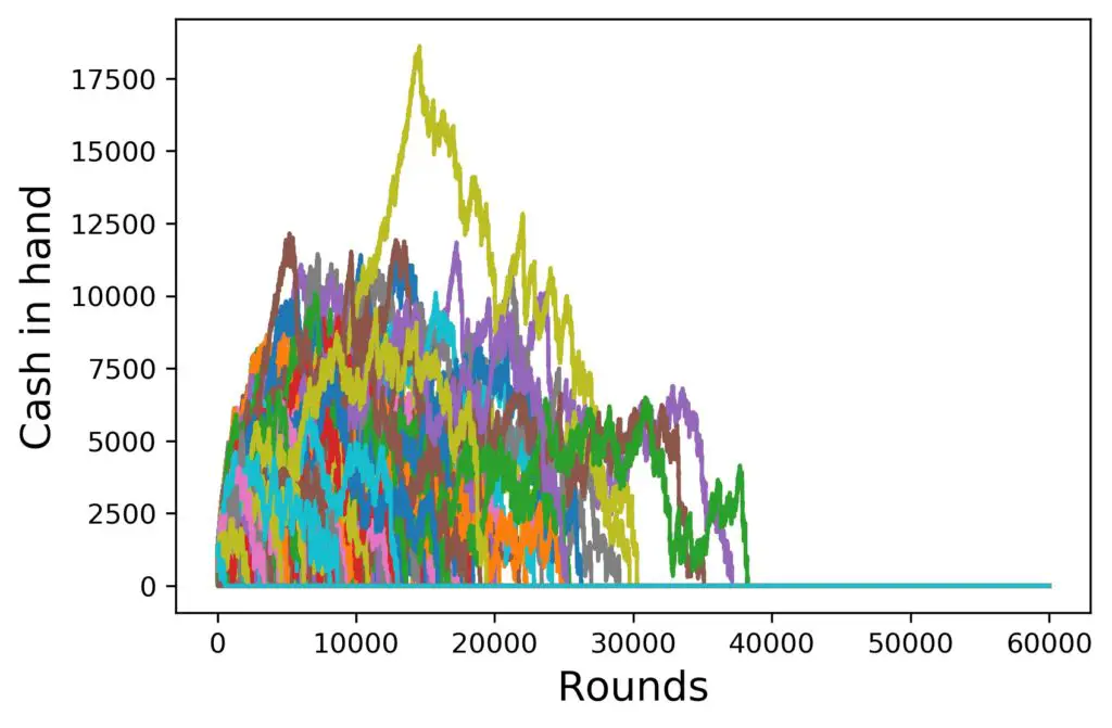
But is it really that bad? Let’s have a look at our 10 000 players, playing the Martingale strategy for 60 000 rounds once again, but this time with a 1000 $ table maximum. Here they are:

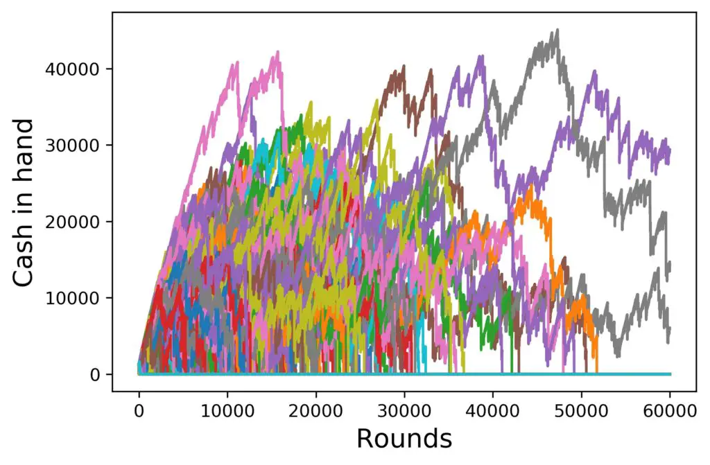
Whoa, now that looks quite a bit different from the graph we just saw before. Observations:

Players still lose it all in all phases of the game.
Some players (in this particular case three out of 10 000) make it to 60 000 rounds and stay alive.
Only very few players get to above 30 000 dollars, ever, for brief periods of time.
The curves lost their nice linear characteristic over the long run.
The curve slope, even for the top ones, has fallen below the 5 $ average win per round.

Ok, now that looks less stellar than just a moment ago in the unlimited fantasy world, right? But we still need to get to some actual numbers for probabilities that we can use, so here we go.

How Long Does it Take to Lose Everything at the Roulette Table With the Martingale System?

Another way of asking this question would be this: how high is the probability of losing everything at Roulette with the Martingale system as after a given number of rounds?

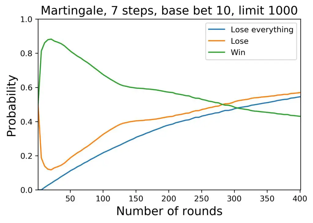
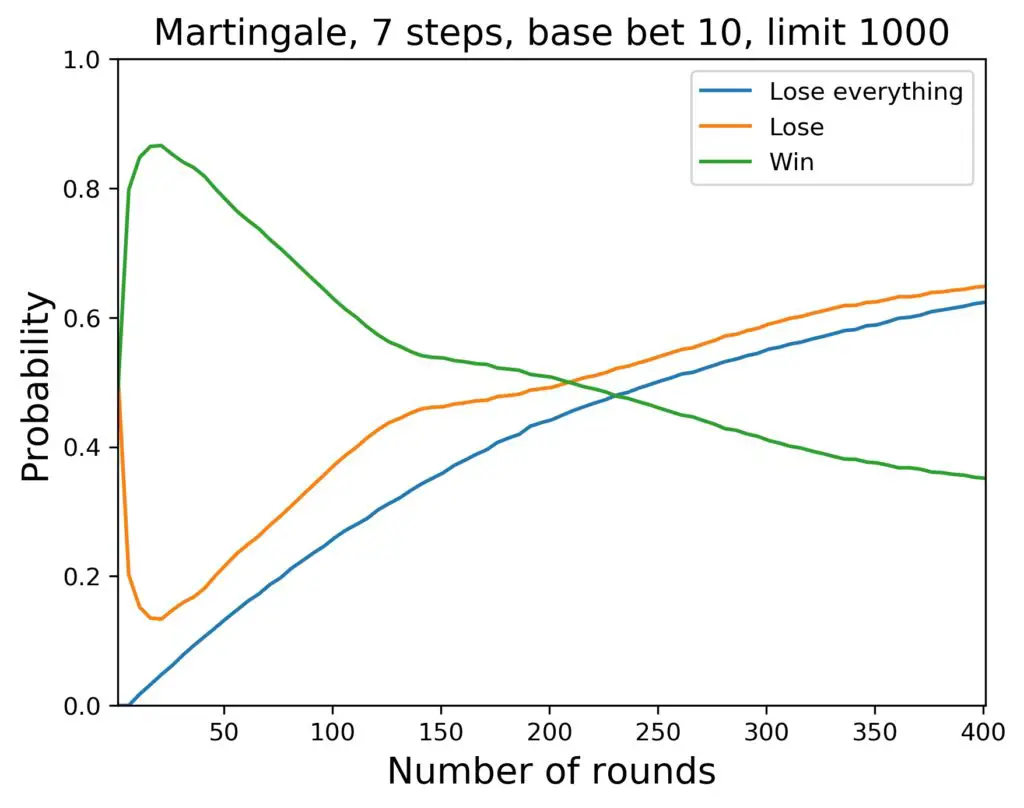
In order to answer that question, I looked at the numbers for cash in hand at each round of the runs and prepared the appropriate means from the samples. Here is the result for the three main probabilities for a 7 step progression in the Martingale system with no table limits. We look at 200 rounds of playing, and the result is based on 200 000 runs:

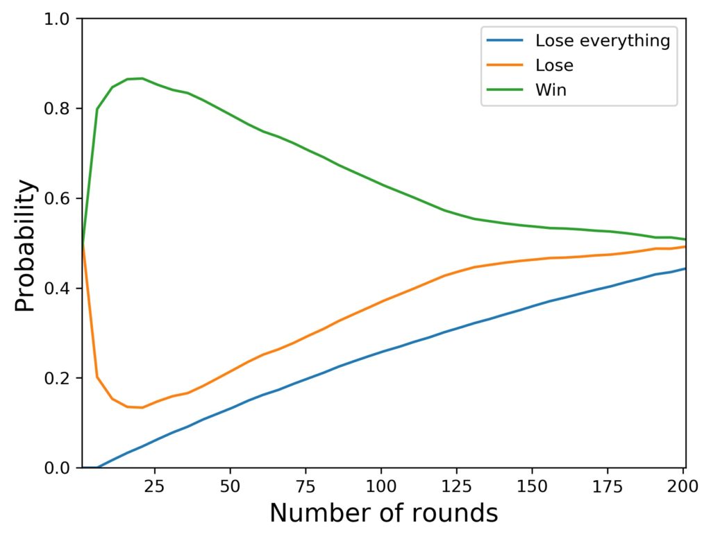
What exactly is shown by these curves? There are three of them:

The green curve shows the probability to be up against the starting amount of cash (in this case 1270 $) by whatever amount. So that could mean that you are up 10 $ or 20 $ or somewhat more – the amount doesn’t matter.
The green curve also includes the rare cases where a player arrives at exactly the starting amount again after so and so many rounds.
The orange curve shows the probability to be down against the starting amount of cash (in this case 1270 $) by whatever amount. This probability includes all sorts of losses, also total loss.
The blue curve shows the probability for a total loss.

Ok, that’s a nice overview, but computed without a table maximum, so let’s look at the difference before we start interpreting the results.

Here is the same graph again, but the simulation was run with a table maximum of 1000 $ (all other parameters are the same: number of samples, samplesize, etc.):

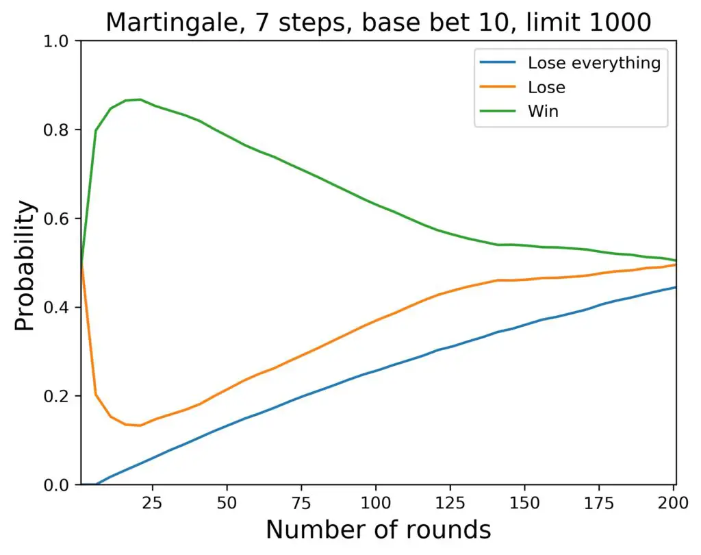
Now, does that actually look any different? Maybe a tiny bit, but that isn’t surprising. We have seen that, in the beginning of the game, a table maximum that matches your size of initial cash does not make a big difference. But how about a lower maximum, say, only 150 $? Then we get restricted to 4 steps in the progression. Can we spot a difference there? Let’s have a look:

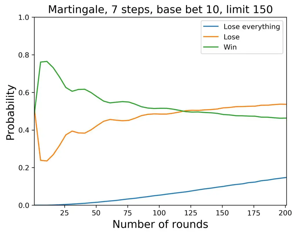
Yes, that looks different, indeed. Probabilities for winning get lower, probabilities for losing go up, while the probabilities for a total loss go down. Probabilities for winning and losing cross much earlier. Can we extract any reasonable statements from these three charts? I’ll give it a try:

Bad things first: a total loss can occur as soon as you have to go all the way up the steps in the progression and that reaches your total amount of cash. As soon as that many rounds have passed, the probability of a total loss keeps rising, and rising, and rising.
For higher table maximum, the probability for a total loss is higher when compared to a lower table maximum. In our example, we reach 44 percent after 5 hours of playing for a table maximum of 1000 $. If the maximum is lower at 150 $, we reach 15 percent total-loss probability “only”.
The probability for losing (net cash change compared to beginning) goes up, when the table maximum is lower, however.
Accordingly, the probability for winning (net cash change compared to beginning) goes down, when the table maximum is lower.
So a high table maximum leads to higher probability to use the Martingale system to your advantage, although a total loss is more likely.
The highest probability for walking away with a win (however small) is found during the first hour or so (couple of tens of spins of the wheel) of playing. After that, the net winning probability goes downhill steadily.
Depending on the table maximum, after a few hours of playing, it is more probable to lose (compared to the beginning) than to win, no matter how much.

How Much Can You Win With the Martingale System for Roulette?

In principle, you can win half your starting bet per round on average with the Martingale System for Roulette. This only holds true, however, if you avoid a total loss.

This question should be approached with caution and a lot of sense for subtleties. In the simulation graphs above we have seen the individual amounts of cash rise and fall for all the simulated players. While most of them were falling, some of them (the luckier ones) went up to several thousands of dollars from a starting amount of roughly one thousand dollars (before they eventually fell to zero, too).

However, when we considered table limits, the behavior of the curves changed dramatically, in particular in the long run. To make things a bit more clear, let us get back to those charts once more. Before, I showed you the long-run characteristics of the simulated curves for a table maximum of 1000 $. Now, I’ll show you the same simulation, but with a lower maximum of 150 $.

The reason is that we have just learned that a lower table maximum reduces both the odds of winning overall and of a total loss. Let’s see how these two work out against each other:

Bam. Now, there is a lot of empty space in the right half of the chart, where there wasn’t for the higher table limit. Furthermore, the curves do not go nearly as high as with the higher maximum.

To compare the two table maxima better, I’ll put both figures up once more, next to each other. Note that the scale on the horizontal axes is the same, but on the vertical axes is quite different:

What we see here is:

The largest wins are in the region of a few tens of thousands of dollars versus barely above 10 000 $. So that’s how much one could win. But let’s keep in mind these occur very rarely and that we are looking at 10 000 simulated players here. Do you feel lucky enough to be one out of 10 000? I don’t.
Keeping in mind that the winning process with the Martingale system is a slow one, and the losing process is a rapid one, it is questionable, how much the average guy can win using this strategy, if at all.

Speaking of the average guy: the average amount of cash that a player has in hand goes down after each round. I haven’t really mentioned this so far, but that is important, too. On average, the players lose, because the probability favors the casino. This is well known, but worth mentioning every now and then. The casino wins, now matter how the players play, due to the so-called house edge. Speaking of which:

Does the House Edge Matter for the Martingale Strategy in Roulette?

The short answer is: not really. But why not? The important circumstance is this that the Martingale strategy is a very particular system which capitalizes on doubling up and has its strength in the short term. The house edge works in the long term, however and affects the short term only a little.

But you don’t have to take my word for it, I can show you the difference. How exactly do we have to set up an experiment like this? The only difference in the simulation concerns the probability of winning a single round. The other parameters can be varied as we just did in order to study various effects of this and that.

So far, I had set the winning probability to 18/37, which is the correct winning probability for a red vs. black or odd vs. even bet in European (or French) Roulette. In order to remove the house edge, I have to set that to 1/2 instead. This also corresponds to flipping a coin or a similar event of chance with fair odds.

Ok, what are the results? Well, here they are for the usual setup (20 samples of 10 000 simulated players each), and a table maximum of 1000 $. We are looking at the same probabilities as above, now plotted out to 400 rounds of playing, without a house edge:

Here is the same simulation, but with the usual house edge (European Roulette):

What do we notice?

As already suspected, the house edge makes a difference in the long term. The crossing point of winning and losing probabilities occurs earlier by a clearly visible amount, if there is a house edge.
The short term appears largely unaffected, in particular the bump of good chance in the first hour of playing.
The characteristics of the curves are very similar, so the house edge has nothing to do, e.g., with the fact that a loss encountered when playing Roulette with the Martingale strategy is most likely a total loss.

I think this brings us to a point where we can begin to summarize the results of this in-depth analysis of the Martingale strategy for Roulette.

Are There Simple Odds for the Martingale Strategy in Roulette?

The odds for the Martingale strategy in Roulette depend on a number of parameters. It is straightforward to provide odds, e.g., for a total loss during a single progression, but it is more involved to provide general odds.

The simple odds for a total loss during a single Martingale progression are given in the table above towards the beginning of this article. They are constructed via multiplying the number for the losing odds with itself as many times as there are steps in the progression. This means that in Roulette, we get for the European variant for the probability of a total loss as a function of the number of steps n

\[p_\mbox{total loss}(n) = \left(\frac{19}{37}\right)^n\]

For our two typical examples of 4 and 7 steps, we get 7 % and 0.9 %, respectively. While this serves as a nice word of warning, it is not all we can do. In the following table, I provide you with the average probabilities for a win (any amount), a loss (any amount), a total loss, as well as the average cash in hand after a variety of numbers of rounds and for different setups, e.g., limits. All numbers are in percent.

Round	Win (any amount)	Loss (any amount)	Total loss	Average cash in hand in $ (starting amount: 1270)
No table maximum, European variant
5	77	23	0	1267
10	84	16	1	1262
20	87	13	4	1252
50	79	21	13	1226
100	63	37	26	1182
200	51	49	44	1114
400	33	67	64	1015
1000	16	84	84	840
No table maximum, American variant
5	75	25	0	1265
10	83	17	2	1254
20	85	15	5	1234
50	76	24	16	1178
100	59	41	30	1096
200	44	56	51	966
400	26	74	71	789
1000	10	90	90	522
Table maximum 1000 $, European variant
5	77	23	0	1267
10	84	16	1	1263
20	87	13	4	1252
50	78	22	13	1222
100	63	37	26	1182
200	51	49	44	1115
400	35	65	62	1007
1000	19	81	81	819
Table maximum 1000 $, American variant
5	75	25	0	1265
10	83	17	2	1253
20	85	15	5	1233
50	76	24	15	1178
100	58	42	30	1094
200	44	56	50	970
400	28	72	70	790
1000	12	88	87	507
Table maximum 150 $, European variant
5	77	23	0	1267
10	77	23	0	1263
20	69	31	0.2	1255
50	58	42	1.5	1231
100	52	48	5	1189
200	46	54	15	1116
400	40	60	32	989
1000	29	71	59	734
Table maximum 150 $, American variant
5	75	25	0	1264
10	75	25	0	1256
20	66	34	0.3	1239
50	54	46	2	1190
100	45	55	7	1111
200	34	63	21	967
400	28	72	43	744
1000	14	86	76	369

With this in hand, we have a nice overview and can easily spot important differences.

The Martingale Strategy for Roulette: Strengths and Weaknesses

After our in-depth analysis of the Martingale strategy for Roulette, we have seen and can summarize the strengths and weaknesses of this system.

The Strengths of the Martingale Strategy for Roulette:

Has relatively high odds of winning (any size of amount) in the first couple of tens of rounds.
This characteristic survives the existence of a table maximum, although a low maximum decreases the winning probability.
The progression system is widely applicable with a reasonable number of progression steps available despite restrictions by upper and lower table limits in actual casinos. One just needs to adjust the base amount accordingly.

The Weaknesses of the Martingale Strategy for Roulette:

You need a somewhat substantial amount of money to start playing. Depending on the steps you want to be able to go in the progression system, this quickly grows, so this system might not be for everyone.
The possibility of a total loss is very real, and its probability keeps rising with the duration of the game.
For high table limits, the probability of losing is almost saturated by the probability of a total loss. What does that mean? It means that if a player loses compared to the starting amount of cash, the loss is most probably total. This effect increases with the duration of the game.
The table maximum in real casinos drastically reduces the possibility of very large wins. Not that we’ll ever get that lucky anyway, but if we did get lucky and win quite a bit, we’d be disappointed by thinking about how much it could have been without a table maximum.
The average wins are small compared to the possible rather immediate losses that can occur.
When the table maximum is reached during the progression, this doesn’t allow the immediate and full recovery in the next round (only for a win, of course). Betting only part of the double-up amount sets the player back to a lower amount of cash, from which he has to recover by making small wins of the base amount, if luck allows him to.

Is the Martingale System Profitable?

Honestly speaking, for some players, the system is profitable in the short term. All players lose everything in the very long term. And until that happens, the average cash in hand (averaged over a large number of players) decreases with every round.

In more Details, we can find the following points regarding the profit made with the Martingale strategy for Roulette:

The most successful time, on average and in terms of probability for a win of any size, is the first hour of playing, roughly speaking.
The longer the game lasts after that, the less profitable the Martingale strategy becomes.
A low table maximum protects players from losing everything compared to a high table maximum
A low table maximum still raises the probability of losing compared to a high table maximum
After enough rounds of playing, all players lose all their money.

The most important thing to understand for me personally was the significant bump in winning probability for the average player during the first rounds of the game. It is obvious to the critical mind that this must be balanced somehow by the drastic nature of the losses – otherwise casinos would lose money in the short term, and ruin the casinos’ business model.

So I investigated this further and did a calculation and investigation of the first few rounds by hand, in a simple spreadsheet. And there I saw everything very clearly: why the probabilities for winning are so high in the beginning, and how the balance of wins and losses works. If you are interested, here is the article: Odds in the Martingale System: Math and Excel Cheat Sheet.

Do with this information here what you will, but I consider this article and analysis a strong warning against playing games of chance for money. If you haven’t already, please read my simulation disclaimer.

What is Reverse Martingale?

If you found this analysis interesting and are also interested in various betting systems, I have another analysis for you. It concerns the so-called Reverse Martingale strategy, which has some important differences. Is that any good? Find out in my article Reverse Martingale for Roulette: Total Disaster or Genius?